An introduction to mathematical modeling in systems biology - MATLAB GUI version
January 2024
v 8.2
Welcome to the computer exercise! In this exercise, you will get a streamlined version of a typical workflow in a systems biology project. You will be introduced to hypotheses of a biological system, and will then formulate models of these to describe experimental data. Then, you will test the different hypothesis to see if you can reject any of them using experimental data, and finally make predictions with the models.
Throughout the lab you will encounter different "admonitions", which as a type of text box. A short legend of the different kinds of admonitions used can be found in the box below:
Different admonitions used (click me)
Background and Introduction
Useful information
Guiding for implementation
Here you are tasked to do something
Reflective questions
Introduction
First thing to do, is to read the introductions "hidden" below.
Click to expand introduction
Purpose of the lab
This lab will on a conceptual level guide you through all the main sub-tasks in a systems biology project: model formulation, optimization of the model parameters with respect to experimental data, model evaluation, statistical testing, (uniqueness) analysis, identification of interesting predictions, and testing of those predictions.
How to pass
To pass the entire lab you need to pass all of the checkpoints. These are marked with Checkpoint x. Please feel free to talk to one of the supervisors if you have any questions regarding any of the checkpoints.
Preparations
Most of the tasks below start with read about .... If one wants to prepare, these can be read in advance of the lab. They are written more as a background about the different topics, and can be read without solving the previous tasks.
Getting MATLAB running
To do the lab, you need access to MATLAB. Depending on if you are using a private computer or one in the computer hall, you need to do either of the alteratives below.
On your own computer
If you don’t already have a Mathworks account, start by making one. If you are a student at Liu you have access to a MATLAB licens via the student portal on LISAM. Go to the Mathworks homepage, download and install MATLAB (version R2018b, or later).
Note that when prompted during the installation, you’ll need to install the Global Optimization Toolbox (version 3.4 or later) and the Statistics and Machine Learning Toolbox.
NOTE that if you are running this computer lab on a mac you might experience unintended bugs or craches. If this occurs it is recomended to run the lab via a remote connection to the universities computer system. See below for how to set up a remote access the universities computers.
If you’re a student at LiU you can remote access the universities computer system via ThinLinc. Note that you need to be connected via VPN to the LiU network before starting ThinLinc. See the link below for more information regarding this (note that page is in Swedish). https://www.ida.liu.se/~TDIU08/UPP_Course_Mtrl/tools/thinlinc/index.sv.shtml
In the university's computer halls
If you are working on a Linux based computer in the computer hall, use the following steps to get MATLAB going.
First, open a terminal. Then run module add prog/matlab/2022a.
Note that the version sometimes changes, if 2022a can't be found, check available versions with module avail or module avail prog/matlab*. This should list all available modules or all available Matlab modules respectively.
Questions?
If you have questions when going through the lab, you can either bring them to the computer lab sessions. You can also raise them on the Q&A page on LISAM. In many situations, your fellow students probably know the answer to your question. Please help each other if possible!
Main computer lab tasks
Model formulation and the experimental data
Getting started
Read about the biological system and experimental data
During the following exercises you will take on the role of a system biologist working in collaboration with an experimental group.
The experimental group is focusing on the cellular response to growth factors, like the epidermal growth factor (EGF), and their role in cancer. The group have a particular interest in the phosphorylation of the receptor tyrosine kinase EGFR in response to EGF and therefore perform an experiment to elucidate the role of EGFR. In the experiment, they stimulate a cancer cell line with EGFR and use an antibody to measure the tyrosine phosphorylation at site 992, which is known to be involved in downstream growth signalling. The data from these experiments show an interesting dynamic behaviour with a fast increase in phosphorylation followed by a decrease down to a steady state level which is higher than before stimulation (Figure 1).
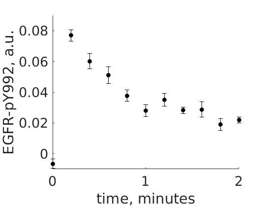
Figure 1: The experimental data. A cancer cell line is stimulated with EGF at time point 0, and the response at EGFR-pY992 is measured
The experimental group does not know the underlying mechanisms that give rise to this dynamic behavior. However, they have two different ideas of possible mechanisms, which we will formulate as hypotheses below. The first idea is that there is a negative feedback transmitted from EGFR to a downstream signaling molecule that is involved in dephosphorylation of EGFR. The second idea is that a downstream signaling molecule is secreted to the surrounding medium and there catalyzes breakdown of EGF, which also would reduce the phosphorylation of EGFR. The experimental group would like to know if any of these ideas agree with their data, and if so, how to design experiments to find out which is the more likely idea.
To generalize this problem, we use the following notation: EGF – Stimulation (S) EGFR – Receptor (R)
Setting up the lab interface
The graphical user interface (GUI) version of the lab is available from here
- Unzip the downloaded file in an appropriate location.
To start the GUI you simply need to run the GUILab.mlapp file in MATLAB (version 2018b or later). There are three ways to do this.
-
If your computer recognises the .mlapp file format, you should be able to simply double click the file to run it in MATLAB.
-
Open MATLAB and navigate to the folder where you have extracted the files. Then either
- Type
GUILabinto the MATLAB command window. - Drag the GUILab file from the folder on the left and drop it in the command window.
- Type
NOTE! If you open simply double-click the GUILab.mlapp file in the MATLAB environment you will open the app development editor. Should this be the case, close this window and open as described above.
The first time you run the lab there will be a slightly longer start up time and there will be a lot of printout in the MATLAB command window. This is the main toolbox installing and is to be expected.
Implementing a simple model
Let's now look at how we can define and simulate a very simple model.
Defining a model
To start with run the GUILab.mlapp file in MATLAB to open the graphical user interface.
To define this model, press the Define Model button, this will bring up a secondary window that allows you to define your models. The components of this window are described below and depicted in figure 1.
- The model text file – This is the primary text area and contains the .txt file that defines the model.
- This drop-down menu contains previously saved models, which can be loaded into the primary text area with the
Load Modelbutton. - This text area displays relevant status text for a compiled or saved model.
- This button compiles the .txt file into an executable MATLAB file, this is necessary for efficient model simulation.
- This button saves the current content of the primary text area to be loadable at a later time. The model will be saved under the name defined under the heading
**********MODEL NAME.
Figure 2 an overview of the Define model window.
Implement the simple example model
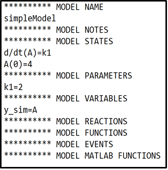
We will start by defining and simulating a very simple model that describes a single state (A). The state A will have an initial value of 4 (\(A(0)=4\)) and will increase at a constant rate of \(k_1 = 2\).
-
Bring up the Define model Window (as described above).
-
Define the simple model as depicted in the box below.
- Under the
**********MODEL NAMEheading, Give the model a suitable name. - Under the
**********MODEL STATESheading, define the derivatives (d/dt) of the model states. Followed by the initial condition of each state. - Under the
**********MODEL PARAMETERSheading, define the initial values of the model parameters. - Under the
**********MODEL VARIABLESheading, here we define what can be measured, also called the measurement equation or \(\hat{y}\). In this model the measurement equation is equal to the amount of state A.
- Under the
- Click the
Compile Modelbutton to compile and save the model.
Simulate your simple model
Now you should simulate this simple model. Start by closing the define model window and return to the main GUI.
- Click the
Update Listbutton to update the list of models in the drop-down menu to include any new defined models. - Select the simple model from the drop-down menu, the model will be listed under the name given during model definition.
- Press the
Simulatebutton, this will simulate the model and plot the observed property \(\hat{y}\) as a blue line. -The slider now labelled k1 can be used to change the parameter value of parameter k1, the model behaviour will change accordingly.

NOTE: the values on the slider are logarithms of 10 i.e. \(1=10^1\). The value in the text field is the actual parameter value.
Does the model behave as expected, given how you defined it? Please take a minute to consider the following questions before continuing.
- How is the initial value \(A(0) =4\) reflected in the plot?
- How is the parameter value \(k1 = 2\), i.e. the rate of change in A, reflected in the plot?
If you are unsure regarding the answers to these questions, feel free to discuss them with another student or a supervisor.
Implementing the first hypothesis
Now that we know how to simulate a simple model, let us implement the hypotheses your collaborators have as models, and simulate them.
Read about the first hypothesis that your collaborators have
To go from the first idea to formulate a hypothesis, we include what we know from the biological system: - A receptor (R) is phosphorylated (Rp) in response to a Stimulation (S) - A downstream signaling molecule (RS) is activated as an effect of the phosphorylation of the receptor - The active downstream signaling molecule (RSp) is involved in the dephosphorylation of the receptor - Phosphorylated/active molecules can return to inactive states without stimuli
From this knowledge, we can draw an interaction graph as depicted in Figure 3, along with a description of the reactions.
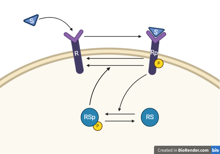
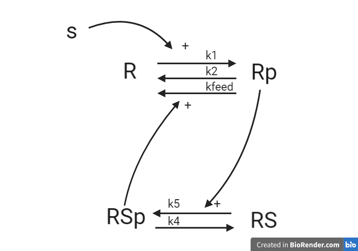
Figure 3: Model 1 – The Feedback Hypothesis. The biological interpretation with the substrate S the receptor R/Rp and the signalling molecule RS/RSp (top). The model interaction graph of the states and the reactions with the corresponding parameters (bottom)
This model will consist of 5 states, 5 reactions with 5 kinetic rate parameters. All reactions are assumed to have mass action kinetics.
- Reaction 1 is the phosphorylation of the receptor (R). It depends on the states R and S with parameter k1.
- Reaction 2 is the basal dephosphorylation of Rp to R. It depends on the state Rp with the parameter k2.
- Reaction 3 is the feedback-induced dephosphorylation of Rp to R exerted by RS_p. This reaction depends on the states Rp and RSp with the parameter kfeed.
- Reaction 4 is the basal dephosphorylation of RSp to RS. It depends on the state RS_p with the parameter k4.
- Reaction 5 is the phosphorylation of RS to RSp. This phosphorylation is regulated by Rp. The reaction depends on the states RS and Rp, with the parameter k5.
The input to the model is the starting concentration of the substrate (S). Finally, the measurement equation is a one to one relationship with Rp, it is defined by the variable y_sim.
Defining the model
Start by defining a model for this hypothesis, in the define model window. To help you get started you can use the template provided below. Note how MODEL REACTIONS can be used to simplify the expression of the state derivatives.
where \(r1 = R*S*k1\) and \(r2=Rp*k2\).
To complete the model in the box below, you will need to:
- Add a suitable model name.
- Complete the equations for states R and Rp
- Add derivatives for states S, RSp and RS.
- Add initial conditions for states S, RSp and RS.
- Define Reactions 3, 4 and 5 as described above.
- Add parameters k4,k5 and kfeed.
- Define the measurement equation for y_sim, as described above.
Note that the derivatives of states R and Rp in the box to below are not complete and needs further additions to accurately correspond to the interaction graph in figure 3.
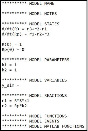
Use the following as initial values for the parameters and the model states.
| Initial values | Parameter values |
|---|---|
| R(0) = 1 | k1 = 1 |
| Rp(0) = 0 | k2 = 1 |
| RS(0) = 1 | kfeed = 1000 |
| RSp(0) = 0 | k4 = 1 |
| S(0) = 1 | k5 = 10 |
Once you are satisfied with the model use the Compile Model button to save and compile the model. Close the window and return to the Main GUI.
Simulate the first hypothesis
- Use the
Update Listbutton to update the drop-down menu. - Select the model for the first hypothesis from the select model drop-down menu.
- Select the data file called
experimentalData.matfrom the select data drop-down menu. You can use theInspect Databutton to the left of the drop-down menu to get a better understanding of the data. - Use the
Simulatebutton to simulate the model for the first hypothesis. - Save the plot of your simulation with the default parameters. Use the
Export Figurebutton in the bottom right corner to export the current plot to a separate window. From this window you can save your figure.

In the main GUI you can now use the parameter sliders to change the corresponding parameter values to see how they affect the model simulation.
- Try to align the model simulation with the experimental data, using the parameter sliders to change the parameter values.
Implement the second hypothesis
Read about the second hypothesis that your collaborators have
The second hypothesis is similar to the first hypothesis and is depicted as an interaction graph in Figure 4. Study this interaction graph and note how it differs from the interaction graph in Figure 3.

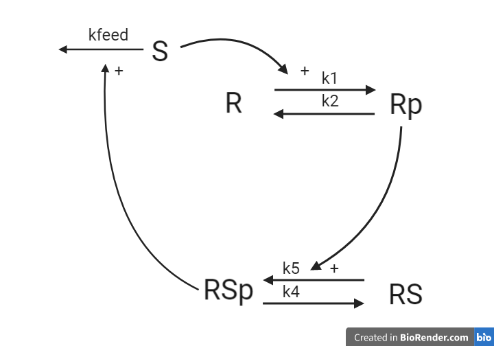
Figure 4: Model 2– The Degradation Hypothesis. The biological interpretation of the second hypothesis with the substrate S the receptor R/Rp and the signalling molecule RS/RSp (top). The model interaction graph of the states and the reactions with the corresponding parameters (bottom)
This hypothesis is similar to the first one, but with some modifications. Here, the feedback-induced dephosphorylation of Rp (reaction 3 in the first model) is removed. Instead we add a feedback-dependent breakdown of the substrate S. This reaction is dependent on the states RSp and S with a parameter kfeed (same name, but a different mode of action).
Define the model for the second hypothesis
To implement this second hypothesis as a model return to the Define Model Window. You can define this model by doing minor changes to your first model and saving it under a different name.
- Load your first model by selecting it in the drop-down menu and clicking the
Load Modelbutton. - Implement the changes necessary for the model to correspond to the hypothesis described above.
- Ensure that you select a different model name for your second model.
- Use the
Compile Modelbutton to save and compile your model for the second hypothesis.
Use the following as initial values for the parameters and the model states.
| Initial values | Parameter values |
|---|---|
| R(0) = 1 | k1 = 5 |
| R_p(0) = 0 | k2 = 20 |
| RS(0) = 1 | kfeed = 10 |
| RS_p(0) = 0 | k4 = 15 |
| S(0) = 1 | k5 = 30 |
Simulate the second hypothesis
- Simulate your second model and save a plot of the simulation with the default parameter values.
- Try to align the model simulation with the experimental data, using the parameter sliders to change the parameter values.
Checkpoint 1: Show your supervisor the plots for both of your models with data, both for the initial parameter values given to you and your best estimation. Also present how you modified the first model to get the second model (show your equations).
Questions to reflect over
- What could be possible reasons why not all states of the model are measured experimentally?
- Was it easy finding a better agreement? What if it was a more complex model, or if there were more data series?
Evaluating and improving the agreement to data
You will have noted by now that the agreement between simulation and data is heavily dependent on the parameter values. But how do we evaluate how good the agreement is quantitatively? We use a cost function.
Read about the cost function
We will now start to address the issue of obtaining parameters that yield a more agreeable fit. We will begin by looking at how we quantify the difference between the simulated and the experimental data. If we have a value that describes how well our simulation, that depends on a set of parameter values, agrees with the data, we can use this value to compare different sets of parameters. Let's call this value the "cost" of a given parameter set.
The cost is computed by the so-called cost function. The cost function is computed by taking the sum of the weighted residuals between the simulation and the experimental data points.
- The residuals are simply the differences be the data points (\(y(t)\)) and the model simulation (\(\hat{y} (t,θ)\)) i.e. \(y(t)-\hat{y}(t,\theta)\).
- These residuals are weighted by the standard error of the mean (SEM) such that data points with large uncertainties contribute less to the cost function value.
The full cost function is formulated as
\(\theta\) is the vector containing the parameter values. \(v(\theta)\) is the cost of the parameters \(\theta\), \(t\) is the time, \(y(t)\) is the experimentally measured mean value at time point \(t\), \(\hat{y}(t,\theta)\) is the model simulated value at time point \(t\), given parameters \(\theta\), \(SEM(t)\) is the standard error of the mean for the data at time point \(t\).
The standard error of the mean essentially describes the uncertainty of a sampled mean value and is calculated as
Where \(\sigma(t)\) is the sample standard deviation of the data at time point \(t\) and \(N\) is the number of observations at time point \(t\).
Try to find a good combination of parameter values
Since we want our model to give an accurate description of our experimental system, we want to find the parameters that minimizes the difference between our experimental data and our model simulation i.e. we want to find the parameters that minimizes the residuals. Since smaller residuals will result in a lower cost (\(v(\theta)\)), the parameters give the most accurate description of our experimental system will be the parameters with the lowest cost.
In the top right corner of the main GUI there is a tick box with the label "show residual", if ticked the plot will show the current residuals.
Next to the "Show residuals" box there is a second tick box, lablled "Show cost function value". When this box is ticked the GUI will display the cost function value for the current set of parameter values at the top of the window.
- Tick the
Show cost function valuebox, in the upper right of the GUI.
To the left ot the "Show cost function value"-tick box there is a drop-down menu with the titel Select a cost function. If you hold the mouse pointer over the question mark to the left of Select a cost function it will display a tooltip with descriptions for different alternative cost functions.
- Read through the descriptions for the different cost functions.
-
Select the cost function you think is most appropriate to use in this situation. If you are unsure, go through the "Read about the cost function" section above once more.
-
For both of your models, use the parameter sliders to try and find the set of parameters that results in the lowest cost.
- You can easily swap between your models via the select modeldrop-down menu.
- Once you have a set you have a set of parameters with a satisfactory low cost use the
Save Parametersbutton to save your parameters.
The Save Parameters button will save the current the parameters using the following naming convention
ParameterValues_[MODEL NAME]_cost([COST VALUE OF PARAMETERS])_[DATE AND TIME].mat
A saved parameter sets can be loaded by selecting it from the drop-down menu and pressing the Load button.
Testing the model with statistical tests
Now that we have a way to quantitatively assess the goodness of a models’ fit to data; it is time to determine if the model fit is good enough.
Read about statistical test to see if you must reject the model
There exist many statistical tests that can be used to reject hypotheses. One of the most common, and the one we will focus on in this lab is the chi-squared (\(\chi^2\)) -test. A \(\chi^2\)-test is used to test the size of the residuals, i.e. the distance between model simulations and the mean of the measured data.
For normally distributed noise, the cost function, \(v(\theta)\), can be used as test variable in the \(\chi^2\)-test. Therefore, we test whether \(v(\theta)\) is larger than a certain threshold. This threshold is determined by the inverse of the cumulative \(\chi^2\)-distribution function. In order to calculate the threshold, we need to decide significance level and degrees of freedom. A significance level of 5% (p=0.05) means a 5% risk of rejecting the hypothesis when it should not be rejected (i.e. a 5 % risk to reject the true model). The degrees of freedom is most often the number of terms being summed in the cost (i.e. the number of data points). In this lab we have 11 data points meaning that the inverse of a cumulative \(\chi^2\)-distribution with a significance level of 5% equals
If the calculated cost is larger than the threshold, we must reject the hypothesis given the set of parameters used to simulate the model. However, there might be another parameter set that would give a lower cost for the same model structure. Therefore, to reject the hypothesis, we must search for the best possible parameter set before we use the \(\chi^2\)-test.
- Given the \(\chi^2\)-threshold of 19.68 and the best model fit you acquired earlier, can you reject either of the two hypotheses?
- Can you be certain that there exists no set of parameters that would generate a lower cost?
Parameter Estimation - Improving the agreement to data
To be able to truly test a hypothesis, we must find the parameters that yield the best possible agreement between data and simulation.
Read about parameter estimation
If the model is not good enough assuming we have the best possible parameters, the hypothesis must be rejected. It is possible to find this best combination of parameters by manually tuning the parameters. However, as you might have discovered this is difficult and could take along time. Instead, we can find the parameters that yield the best agreement using optimization methods.
An optimization problem generally consists of two parts, an objective function with which a current solution is evaluated and some constraints that define what is considered an acceptable solution. In our case, we can use our cost function as an objective function and set lower and upper bounds (\(lb\)/\(ub\)) on the parameter values as constraints. The problem formulation typically looks something like the equations below.
where \(\theta^*\) is the optimal set of parameters that minimizes the cost function \(v(\theta)\). An optimization problem can be hard to solve, and the solution we find is therefore not guaranteed to be the best possible solution. We can for example find a solution which is minimal in a limited surrounding, a so-called local minimum, instead of the best possible solution – the global minimum. There are methods to try to reach the global minimum, for example you can run the optimization several times from different starting points and look for the lowest solution among all runs. Please note that there might be multiple solutions with equal cost values.
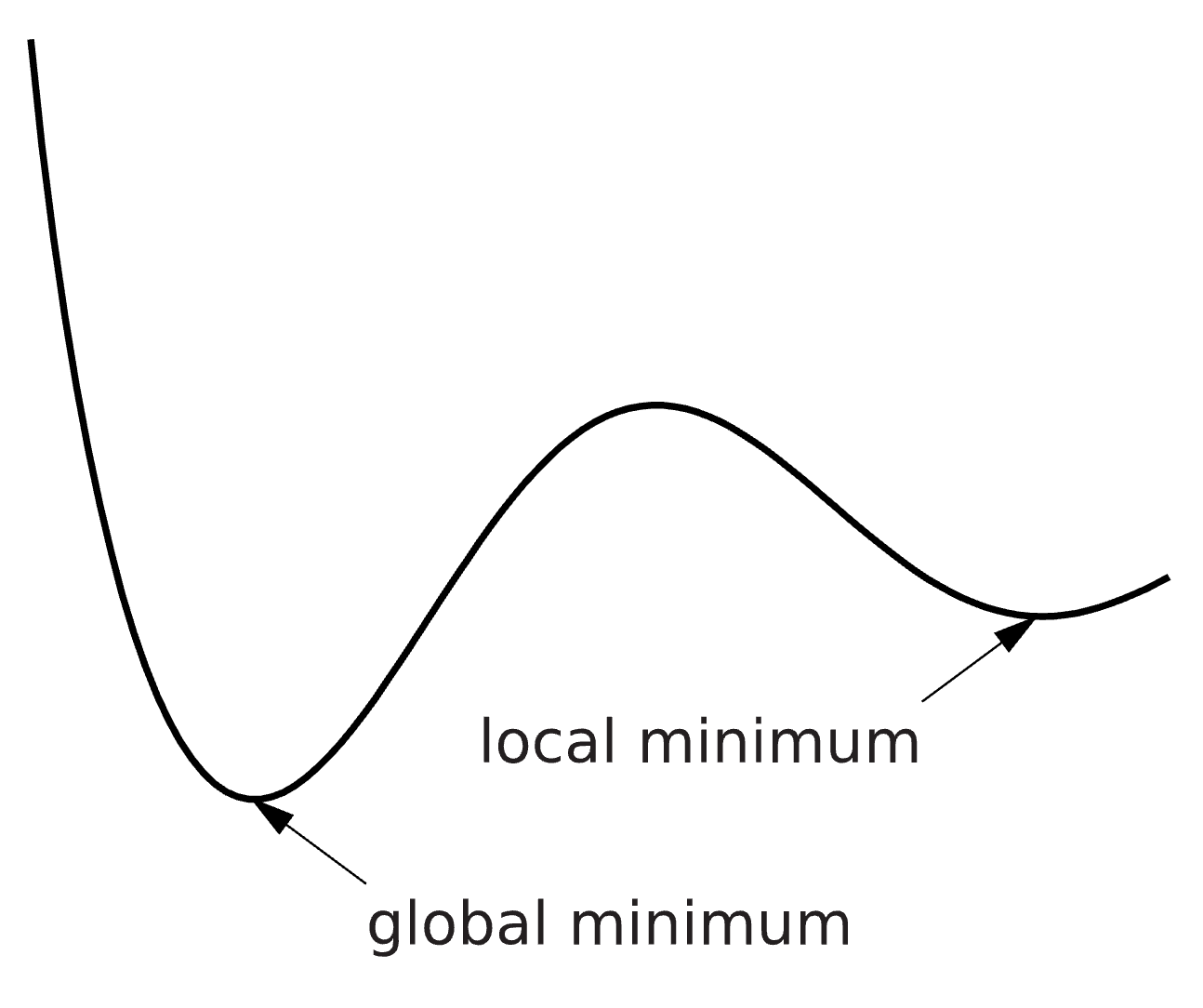 *Figure 5: An Illustration of the objective function landscape that is explored during optimization. With the difference between local and global minimum illustrated.
Estimate the parameter values, for both of your models
In the main GUI you can use the Optimize Parameters button to run an implemented optimization algorithm for the currently selected model and experimental data. The optimization algorithm will search for a set of parameter values that minimizes the currently selected cost function, starting with the currenly set prameter values. Note that the optimization process will take several minutes to complete. Once completed the optimal parameters will be presented on the parameter sliders and the plot will update to plot the optimal solution.
- For each model, click the
Optimize Parametersbutton to initiate the optimization algorithm. The optimization will take about two minutes to complete (might be faster).
Note also that there is no guarantee that the optimization algorithm will return the same value every time it is run. Running it again might return an even better parameter set with a better cost value. Further, the optimization algorithm will use the current parameter values as an initial guess i.e. subsequent optimizations is more likely to result in better solutions.
- To ensure that we find the best possible solution, run multiple optimizations for both models.
- Remember that you can use the
Save Parametersbutton to save a found parameter set before running a new optimization.
- Remember that you can use the
- For each model, save the plot of the best solution you found, using the
Export Figurebutton.
(spoilers) Self-check: How do I know if I have found a good enough solution?
Both models should be able to reach cost values below 20.
Checkpoint 2: Which model has the best fit to the data in terms of the lowest cost? Could either model be rejected? Plot the optimal fits of both model to the experimental data and show your results to your supervisor. Briefly describe the cost function: What are the residuals? Why do we normalize with the squared uncertainty?
Questions to reflect over
- Why do we want to find the best solution?
- Are we guaranteed to find the best solution?
- Do you reject the first hypothesis?
- If you did not reject the model, how can you test the model further?
Using the model to make predictions
Now that we know whether our models should be rejected or not, given the solution from our optimization algorithm, it is time to estimate the uncertainty of our models.
Read about how we can estimate the model uncertainty
After the optimization procedure, we decide if the hypothesis should be rejected or not. If the best cost value is lower value than the \(\chi^2\)-threshold, we will move on and further study the behaviour of the model. Unless the best solution is strictly at the boundary, there exists worse solutions i.e. solutions with a higher cost, which would still be able to pass the statistical test. We will now look at all these acceptable solutions. In this analysis, we study all found parameter sets that has a cost lower than the \(\chi^2\)-threshold i.e. all parameter sets that give an acceptable agreement between model simulation and experimental data. These parameter sets are used to simulate the uncertainty of the hypothesis given available data. This uncertainty can tell us things like: Do we have enough experimental data in relation to the complexity of the hypothesis? Are there well determined predictions (i.e. core predictions) to be found when we use the model to simulate new potential experiments?
Since we know the \(\chi^2\)-threshold for our experimental setup, each time we evaluate a parameter set \(\theta\) we can also check if the cost for that parameter set is lower than the \(\chi^2\)-threshold. If it is, we simply save that parameter set.
please note that this is not a completely reliable estimation of the model uncertainty but rather a minimal estimation of the model uncertainty. A true uncertainty estimation is a much larger and more time-consuming analysis. Hence, in this introductory computer exercise this underestimated model uncertainty will be considered good enough.
Estimate the uncertainty for your models
In this lab the model uncertainty will be estimated from a set of acceptable parameter values. During the optimization process the GUI has automatically saved the acceptable sets of parameters that was encountered. However, this results in a very long list of acceptable parameter values. Therefore, you will need to sample a subset of acceptable parameter values to estemate the model uncertainty.
In the botom left corner of the GUI there is a drop-down menu that allows you to select between different sampling approaches. If you hold the mouse pointer over the question mark, the tooltip will describe the differnet approaches. You can also set the number of sampels that will be drawn by your selected approach in the box to the right of the drop-down menu. - Select a suitable sampling approach from the drop-down menu. - Set a suitable number of samples to use for you uncertainty estiamtion.
You can now use the Plot Model Uncertainty button at the bottom of the GUI simulate and plots the simulations for the sampled parameter sets, giving you the model uncertainty.
Known bugs
- If the "Plot Model Uncertainty" button is used with the "Show residuals" box ticked it will cause an "Dimensions of arrays being concatenated are not consistent."-error. Solution: Untick the "Show residuals" box and click the "Plot Model Uncertainty" again.
- If the "Plot Model Uncertainty" button is used without having found an acceptable in the preceding optimization it will cause an "Empty format character vector ..."-error. Solution: Run additional otpimizations and click the "Plot Model Uncertainty" again.
The estimated model uncertainty is really a cmbantion of many differnet simulations, and each simulation can be plotted as a seperate line. However, as you might notice such a plot can be quite messy, one alternative is to combine all of these lines into a shaded area that represents the total uncertainty. You can use the tick box ate the bottom of the GUI to plot the uncertainty as a sahded area
For each model respectively
- Use the
Plot Model Uncertaintybutton at the bottom of the GUI to plot your model uncertainty. Note that this might take some time to complete, depending on the number of samples used. - Experiment with differnt combinations of sampling approaches and Number of Samples to see how they affect the estimated uncertainy. You can always save your plots for comparrison with the Export Figure button, at the bottom right of the GUI.
-
Once you have tried a few sampling approaches and number of samples, and you have found a combination that you feelgives a good estimation of the model uncertainty. Click the Save model uncertainty button. This saves the sampled parameter sets to be used later.
-
Use the
Save Model uncertaintybutton to save the estimated uncertainty. This is required for a later step of this lab. - The Uncertainty will be saved with the following naming convention
SampledParameters_[MODEL NAME]_[DATE AND TIME].mat
Note the file name of your saved model uncertainty as you will need to select it later.
- Save your plot with the model uncertainity, using the
Export Figurebutton
Self-check: Make sure that your uncertainties are not overly narrow. If they are, collect some more parameter sets. If you are uncertain, talk to a supervisor.
Making predictions
Now that we have an estimation of the model uncertainty, it is time to make predictions of new experiments.
Read about predictions
A good model cannot only explain estimation data, it can be used to generate good predictions for new set of circumstances. In order to see if the model is behaving reasonably, we want to see if we can predict something that the model has not been trained on, and then test the prediction with a new experiment. Note that for the prediction to be testable, it must be limited in at least one point, often referred to as a core prediction. A core prediction could for example be found at one of the model states where we do not have experimental data, or at the model state we can measure, under new experimental conditions (extended time, a change in input strength etc.).
Core predictions are well determined predictions that can be used to differentiate between two models. Such a differentiation is possible when model simulations behave differently and have low uncertainty for both models. Core predictions are used to find experiments that would differentiate between the suggested hypotheses and therefore, if measured, would reject at least one of the suggested hypotheses. The outcome could also be that all hypotheses are rejected, if none of the simulations agree with the new experiment.
Use your models to predict the outcome of a new experiment
In this lab we will use our models predict what happens if we introduce additional substrate (S) to the system at a second timepoint. The current interpretation for both of your models is that substrate is only introduced at the start of the experiment, \(t=0\), i.e. \(S(0)=1\).
To model the introduction of additional substrate you will need to modify your model definitions. You will need to introduce something called events, which causes something to happen once a given condition is fulfilled. The something we want to happen is that new substrate is added i.e. our state \(S\) is set to be equal to \(1\). The condition for this should be that the time \(t\) is equal some given time point e.g. \(t=4\)
The above described event would be implemented in your model file like this:

where \(event1\) is the name of the event, \(gt(time,4)\) states that we want the event to trigger at time \(t=4\), S defines that we want to change the value of state \(S\), and the \(1\) at the end defines that we want to change the value of state \(S\) to one. Note that the event is implemented under the ***********MODEL EVENTS heading.
- Open the model definition window with the
Define Modelbutton. - Load your model by selecting it from the drop-down menu and clicking the
Load Modelbutton. -
Add an event that introduces new substrate as described above.
- You are free to choose the time point of the new substrate, the \(t=4\) in the example above is selected for demonstration purposes.
- Use the
Compile Modelbutton to save and compile your modifications. - Repeat the above steps for your second model.
Note that it is important that the event is identical for both models since we want to compare them, and a comparison is only meaningful given identical conditions.
- Return to the main GUI and click the "Model predictions` tab in the top right of the window, to sawp to the Predictions window
In the prediction window
- Select your first model and the file with the corresponding estimated parameter uncertainty that you saved before, from the respective drop-down menus.
- Select your second model and the file with the corresponding estimated parameter uncertainty that you saved before, from the respective drop-down menus.
- Enter a suitable time length of the simulation, if you choose to add substrate at e.g. \(t=4\) then a suitable time length of simulation could be 6 s. this ensures that your simulation encompasses the response to the new substrate.
- Click the
Simulate Predictionsbutton to simulate your predictions. Note that the time to simualte the models will again depend on the number of sampled parameter sets used in the saved files.
Make sure that you have selected the correct parameter files for your respective models.
- Can you identify a core prediction that can be used to distingush between the two hypotheses?
- Would you suggest that this experiment, i.e. adding substrate at a second time point, is performed?
Self-check: Make sure that you can find a prediction where the model predictions are certain, and where the models are behaving differently.
Experimental validation
Read about how we can use experimental validation
The last step of the hypothesis testing is to hand over your analysis to the experimental group. Any core predictions that discriminate between Model 1 and Model 2 should be discussed to see if the corresponding experiment is possible to perform. Now it is important to go back to think about the underlying biology again. What is the biological meaning of your core predictions? Do you think the experiment you suggest can be performed?
Once we have established that the experiment we predicted can be performed and is of value the experimental collaborators will do so and collect new experimental data. This data can be used to validate our models or to discriminate between two competing models.
Experimental validation
In this exercise you can use the Generate new data button in the Prediction window to acquire this validation data. But first you will need to define at which time point you choose to add additional substrate. It is important that this time point correspond to the timepoint you choose when defining the events for your predictions.
Enter the time point at which additional substrate is added.
Click the Generate new data button to generate data from the new experiment.
Save your figure with both your predictions and the new data, using the Export Figure button.
What would you conclude by comparing the simulations of your hypotheses to the validation data?
Checkpoint 3: Show a supervisor your figure with the predictions and the new data. Can you reject any of the hypotheses? Provide short answers for the questions below.
Questions to reflect over
- Did you reject any of the models?
- What are the strengths of finding core predictions, that are different between models potentially describing the same system?
- What is the downside to choosing points where there is an overlap between the model to test experimentally, even if the predictions are certain ("narrow")?
- What would be the outcome if it was impossible (experimentally) to measure between 2 and 3 minutes?
- Is our simulation uncertainty reasonable? Is it over- or underestimated?
- What could be problems related to overestimating the uncertainty? To underestimating the uncertainty?
- What should you do when your model can correctly predict new data?
Summary and final discussion
To concludes this computer exercise, we will look back upon what you have done. Below are some questions to discuss with the supervisor. These questions are all points that have been covered in this lab, if you are unsure about any of the answers go back and look through the corresponding section.
Checkpoint 4: Discuss the questions below with a supervisor. Think if you have any additional questions regarding the lab or Systems biology and feel free to discuss this with a supervisor
Some summarizing questions to discuss
- Look back at the lab, can you give a quick recap of what you did?
- Why did we square the residuals? And why did we normalize with the SEM?
- Why is it important that we find the "best" parameter sets when testing the hypothesis? Do we always have to find the best?
- Can we expect to always find the best solution for our type of problems?
- What are the problems with underestimating the model uncertainty? And with overestimating?
- If the uncertainty is very big, how could you go about to reduce it?
- Why do we want to find core predictions when comparing one or more models? What would be the outcome if one did the experiment?