Lab 4: AI and hybrid modelling¶

The purpose of this lab is to get an overview of different types of models and usages of AI models in health care and biology. You will also learn how different kinds of models can be combined in hybrid model schemes.

Throughout the lab you will encounter different "admonitions", which as a type of text box. A short legend of the different kinds of admonitions used can be found in the box below:

Different admonitions used (click me)

Background and Introduction

Useful information

Guiding for implementation

Here you are tasked to do something

Reflective questions

Before you start with this lab, you are expected to have:

Matlab running on your computer (or a computer in the computer hall)
A C-compiler installed in Matlab
Downloaded and installed IQM tools in Matlab
Downloaded and extracted the scripts for Lab 1.1: Lab1.1 files

If you haven't done this, go to Resources and follow the instructions before you start with this lab.

All files needed in this example can be downloaded at Lab4 files.

How to pass (Click to expand)

At the bottom of this page you will find a collapsible box with questions. To pass this lab you should provide satisfying answers to the questions in this final box in your report. Throughout this lab you encounter green boxes marked with the word "Task", these boxes contain the main tasks that should be performed to complete the lab. There are five tasks in total, and for each task there are questions (found at the end of this page) that should be answered in the report. The questions can be answered in a point-by-point format but each answer should be comprehensive and adequate motivations and explications should be provided when necessary. Please include figures in your answers where it is applicable.

Automized image processing¶

Modelling usually need a lot of data to be useful, especially in different kinds of image analysis - a common usage of AI. When using imaging data, the data usually have to be processed in different ways before it can be used. This preprocessing of data is often time consuming to do by hand.

In this part of the lab, you will process training data for a mathematical model using a deep learning network. More specifically, you will use the deep learning network to automatically segment the heart chambers in 4D flow MRI images, and then use this segmented data to train a cardiovascular mechanistic model describing the left ventricle.

Requirements in MATLAB:

* Simulink
* Simscape
* Simscape electrical
* Curve Fitting Toolbox
* Simulink Design Optimization
* Image Processing Toolbox
* Optimization toolbox
* Global optimization toolbox

To run the deep learning network, python is needed. See "Set up a python virtual environment" in the Task 1 box below, or look into the instructions in the resources tab.

Task 1: Run the DL network to get a segmentation of the left ventricular volume

Download the network
Run the network on the data in the folder 'DLnetwork/Data/ExampleSubject'
Plot and analyze the resulting segmentations

The deep learning network

Segmenting the whole heart over the cardiac cycle in 4D flow MRI is a challenging and time-consuming process, as there is considerable motion and limited contrast between blood and tissue. To speed up this process, this deep learning-based segmentation method was developed to automatically segment the cardiac chambers and great thoracic vessels from 4D flow MR images. A 3D neural network based on the U-net architecture was trained to segment the four cardiac chambers, aorta, and pulmonary artery. Since deep neural networks learn most of there structure from the data, without using any a priori knowledge, they can be called machine learning models.

For more information, see the paper by Bustamante et al: Automatic Time-Resolved Cardiovascular Segmentation of 4D Flow MRI Using Deep Learning.

Download the network

The network is found here: dl-3d-cardiovascular-segmentation. Download it to your computer and put it in your 'DLnetwork' folder. One way to do that without using git is to download it as a .zip file, and then extract it.

Set up: python virtual environment

The python requirements for the network are in the 'requirements_pyenv.txt' file.

Create a python environment on a windows computer:¶

Open Windows Powershell
Go to the lab folder 'DLnetwork' by using 'cd ' and the path to the folder.
Run 'python -m venv pythonenv' to create a python environment in the pythonenv folder.
Run '.\pythonenv\Scripts\Activate.ps1' to activate the python environment. (if you cannot do this, change the settings by running: 'Set-ExecutionPolicy -ExecutionPolicy RemoteSigned -Scope CurrentUser')
Run 'pip install -r requirements_pyenv.txt' to install all requirements inside the environment.

Run the network

To run the network in MATLAB, open the 'DLnetwork' folder in matlab. Read the README-file to get a better understanding of all the files.

Run initialize.m. Then, write DLseg_gui in matlab's command prompt to start the GUI. In the GUI, navigate to and select the folder Data/ExampleSubject. Click the 'Single dataset' checkbox, and press 'Next' to run the network.

Note: the network could take around 10 minutes to run on a normal laptop. You can see the progress in the matlab command window. You can also run the network by running python_scripts/run_inference.py alone, after loading the data using the first step in the matlab gui.

If you cannot get the network running, ask the lab supervisor or another student to get the resulting segmentations to be able to continue with the lab.

Plot the resulting segmentations

Run plotSegmentationResult.m.

Look at the segmentation results.

Do you think the segmentation is correct? Why?
Does the left ventricular volume seem reasonable? Why?

Task 2: Run the cardiovascular model to simulate the left ventricular volume during a heart beat

Do a model simulation
Plot the model simulation of the ventricular volume together with the deep learning-based ventricular volume

The cardiovascular model

Figure 1: The cardiovascular model including the left ventricle.

The cardiovascular model here is an expanded version of the model you used in the model formulation lab. Instead of a sinus wave-based input to the aorta, a left ventricle is added which contracts and relaxes to create a more realistic outflow to the aorta.

This cardiovascular model is formulated in Simulink instead of in DAEs. In the background, matlab translates the model to equations and solves them, but the Simulink interface allows for a drag-and-drop setting when creating the model.

Simulate and plot the model simulations

Find the saved .mat file that contains the left ventricular volume from the segmentation, and put it in the same folder as mainVentricularModel.m.

The simulation process is slightly different in Simulink, and you are therefore given the scripts for simulating the model and plotting the results. Run mainVentricularModel.m in the folder Cardiovascular_model to simulate and plot the model simulations. Note that it might take a few minutes for the program to start.

Look at the plot of the model simulation and the data.

Can the model describe the data?
What is the aortic pressure? Is it reasonable? Why/why not?

Task 3: Fit the cardiovascular model to the segmentation-based left ventricular volume

Optimize the model parameters to fit the left ventricular volume to data.
Plot the resulting simulations of left ventricular volume compared to data, and the predicted aortic pressure.
Note the diastolic and systolic pressure - these results will be used in the next task.

Optimize parameters to fit to left ventricular data

Open parameterEstimation.m in the folder Cardiovascular_model. Choose an optimization solver from the Parameter estimation lab and add a call to it and its settings in the marked places in the script, and then run the parameter estimation. Note that the optimization might take some time.

The downside of Simulink models is that they are a bit slower to simulate than ODE models formulated in IQM toolbox. To speed up the optimization, you can for example: * Only estimate the values of the model parameters governing the contraction and relaxation of the left ventricle (Emax_LV,Emin_LV,k_diast_LV,k_syst_LV,m2_LV,m1_LV,onset_LV) by adapting the toOptimize index. * Set a max time (MaxTime) and/or max number of objective function evaluations (MaxFunctionEvaluations) in the optimization solver settings to make sure that it does not take too long time. * Set more narrow lower and upper bounds for the parameter values. Note that these suggestions are optional.

Look at the plot of the model simulation and the data.

Can the model describe the data?
What is the aortic pressure? Has it changed? Is it reasonable?
Do you think that the data of the left ventricular volume is enough to be able to reliable predict the aortic pressure?
Do you think that the model complexity is good for this amount of data, or could it be smaller or bigger? Look at Figure 1 and discuss.

Impute data¶

Missing data is commonplace in health care. Data could be missing due to cost (some measurement techniques are more expensive than others), measurement errors, lack of compliance, etc. When doing statistical analysis on data with a lot of missing data, the results can be biased or less representative. One way of handling the problem of missing data is to do an imputation, i.e. replacing missing data with substitute values.

In this part, you will impute the missing data in database.mat using k-nearest neighbors (kNN).

Task 4: Impute patient data using kNN

Open the map Impute_data. Before you impute the data, set the systolic and diastolic pressure for the patient on row 1 to the values obtained from task 3 - this will now be referred to as Patient 1. You can do this manually, changing the values in database.mat. Remember to save. In the file Impute.m, set the parameter k (you can read about the parameter k below), and use readtable to load the data for patient 1 and writetable to save the data for patient 1 and the imputed database. Then run Impute.m

Try and compare the resulting imputed data for some different k's and chose one that you think gives reasonable results.

k-nearest neighbors (kNN)

kNN is an algorithm that assigns a class or value to new data points based on their k number of nearest neighbors. The kNN model has one parameter and one equation that has to be decided. The parameter is the parameter k - how many nearest neighbor the classification will be based of. A small value of k means that any data noise will have a higher influence on the results. A large value of k make it computationally expensive and makes the prediction less precise, since you include neighbors that are more dissimilar in the prediction. So the choice of k ultimately depends on your data set. These kinds of parameters that impact the effect of model learning are called hyperparameters, and can also be optimized. The equation that has to be chosen is the distance metric - how the distance to each neighbor is calculated. Two common distance metrics for continuous variables are Euclidean or Mahalanobis distance. Both these distance metrics use the Pythagorean theorem to calculate the distance, but Mahalanobis also accounts for correlation between variables, making it more suitable for datasets with more than two variables. Herein we will therefore use the mahalanobis distance.

Figure 2: Example of kNN classification. The test sample (green dot) should be classified either to blue squares or to red triangles. If k = 3 (solid line circle) it is assigned to the red triangles because there are 2 triangles and only 1 square inside the inner circle. If k = 5 (dashed line circle) it is assigned to the blue squares (3 squares vs. 2 triangles inside the outer circle).

database

A prospective cohort of mostly diabetics and prediabetics.

Variables	Description
AGE:	in years
SEX:	coded as 1 = male 2 = female
BMI:	(kg/m^2) body mass index, calculated as weight/height^2
	<18.5 – underweight
	18.5 - 24.9 – normal weight
	25 - 29.9 – overweight
	0 - 34.9 – obese
	35< - extremely obese
CPD:	average cigarettes smoked per day
DBP:	diastolic blood pressure in mmHg. The diastolic blood pressure is the lowest pressure during the heart cycle, measured when the heart is refilling with blood.
	90 - 120 – normal
	120 - 129 – elevated
	130-139 – high, stage 1
	> 140 – high, stage 2
	> 180 – hypertensive crisis
SBP:	systolic blood pressure in mmHg. The systolic blood pressure is the highest pressure during the heart cycle, measured when the heart is contracting.
	60 - 80 – normal or elevated
	80 - 89 – high, stage 1
	> 90 – high, stage 2
	> 180 – hypertensive crisis
DMRX:	diabetes diagnosis, coded as 0 = no diabetes 1 = diabetes
AF_beforestroke:	atrial fibrillation diagnosed before stroke coded as 0 = no atrial fibrillation and 1 = atrial fibrillation
STROKE:	stroke, coded as 0 = no stroke, 1 = stroke

Look at the imputed data

How could k be chosen in a better way? What would you need to do that?
Can you think of any other type of model you could use to impute this data?
Compare patient 1 with all other patients - can you see any problem with using this specific dataset to impute data for patient 1?

Calculate disease risk¶

Estimating disease risks is an integral part of preventative health care. Things that affect an estimated risk are which risk factors you include, and what algorithm if any you use to calculate it.

Task 5: Calculate the current risk of getting a stroke within 5 years for patient 1

Try to calculate the stroke risk for patient 1, using the data you just imputed, in 3 different ways: i) looking at the imputed value of stroke for patient 1 from Task 4, ii) using the Framingham risk score , and iii) using an ensemble risk model.

Framingham risk score

You can calculate the risk score using this web based calculator: Framingham Risk Score for Hard Coronary Heart Disease. Note that you don't have all the data that the calculator asks for.

run Ensemble risk model

Go to Posit cloud, login or sign up for the free cloud version. Once logged in, click “New Project”, then “New Rstudio Project”. In the “Files” window, in the lower right corner, click the upload button, and the chose file button to upload the files in the map Calculate disease risk and the imputed data file for patient 1 that you saved in task 4. Open the script ensemble_age_model.R by clicking on it in the Files window, and add the file names of your patient 1 data and the name you want to save your results as where it is indicated in the code. Then run that script by pressing Ctrl+Shift+Enter or by clicking Source. Then, open plotRisk and add code to load your results from ensemble_age_model.R as well as the data for patient 1 to the script, and then run the script. You can also add legend text at the end of the script if you want. Note that you will use this model again in a later task.

Ensemble model

Ensemble models use multiple learning algorithms to obtain better predictive performance than could be obtained from any of the used learning algorithms on their own. This specific ensemble model is a combination of logistic regression model for 4 different age groups: under 50, 50-59, 60-69 and over 70. These age-specific models capture the non-proportionality of risk factors by age and are better calibrated to the younger and older populations. By combining the age-specific models into one ensemble model we get a smooth transition of how risk changes over the years. You can read more about this risk model in Age Specific Models to Capture the Change in Risk Factor Contribution by Age to Short Term Primary Ischemic Stroke Risk and in Digital twins and hybrid modelling for simulation of physiological variables and stroke risk.

Compare the risks of the different models

Which of these predictions do you find most useful and trustworthy?
What pros and cons do you see with the different prediction models?

Task 6: Calculate current risk for Patient 2

Come up with values for an imaginary patient 2 that is the same age as patient 1 that you think would give a lower risk of stroke than for patient 1 (you can e.g. copy your patient 1 file, and change the name of the file you load in the scrip). Calculate the risk for patient 2 using the ensemble model, and try out different variable values until you have a patient 2 that has a lower risk of stroke than patient 1.

Compare the risks of the different patients

What do you think is the biggest contributor to disease risk in patient 1 and patient 2's age group?

Simulating scenarios¶

Managing disease risks involves predicting the evolution of risk factors over time, as well as predicting the individual effects of different interventions, such as changes in lifestyle, diet, drugs, etc. One way of doing such predictions is by using mechanistic models.

Task 7: Simulate scenarios using a multi-level mechanistic model

Simulate three scenarios based on patient 1 and patient 2 with the mechanistic model. Simulate for 10 years or longer. Try to come up with scenarios you think would lower the risk for patient 1 and increase the risk for patient 2 over time. Then, at around half of your simulation time, add some intervention to patient 2 so that the risk decreases. You should then have a plot of three scenarios.

Mechanistic model

The mechanistic model is a multi-level multi-time scale, meaning that it consists of several biological levels - in this case cell-, organ/tissue-, and whole body-level -, and that it can be simulated on different time scales - from minutes up to years. The model consist of two parts. One part of the model describes processes relevant to glucose regulation - in a fat cell and in relevant organs during a meal, changes in weight due to diet and subsequent changes in insulin resistance. The model can also get diabetes. The model takes change in energy intake (dEI) in kcal as input. A normal daily intake consists of about 2000-2500 kcal. The model can handle/has been evaluated on a dEI of >250 and 4000> kcal dEI. The other part describes changes in systolic and diastolic blood pressure due to aging and blood pressure medication. It is not as detailed or as individualized as the cardiovascular model in Task 2 and 3, but it can be simulate for longer time periods. You can read more about the model at Digital twins and hybrid modelling for simulation of physiological variables and stroke risk and A multi-scale digital twin for adiposity-driven insulin resistance in humans: diet and drug effects

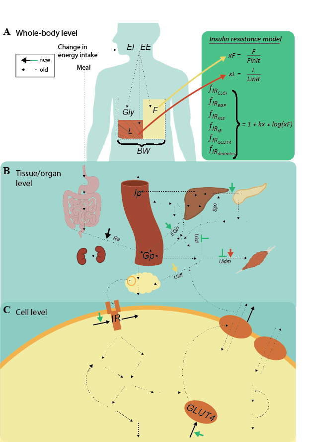
Figure 3: Overview of the diabetes part of mechanistic multi-level model. A) Whole-body level. The body composition model takes change in energy intake as input, i.e., the difference in energy intake (EI) and energy expenditure (EE). This difference translates to the outputs: changes in the masses of fat (F), lean tissue (L), and glycogen (Gly). The total sum of these masses is the body weight (BW). The insulin resistance model (green box) takes the change in fat mass (xF) as input. B) The following factors influence the glucose concentration on the tissue/organ level: the insulin resistance, xF, the change in lean tissue (xL), and BW. More specifically, insulin resistance (green short arrows) increases endogenous glucose production (EGP) and insulin secretion (Ipo), and decreases glucose uptake in both muscle (U_idm) and liver tissue (U_idl). Furthermore, xL increases U_idm, xF increases glucose uptake in fat tissue (U_idf), and BW increases the rate of appearance of glucose (Ra). C) Finally, the amount of insulin in fat tissue translates to insulin input on the cell level. More specifically, insulin binds to the insulin receptor (IR), causing a signaling cascade that ultimately results in glucose transporter 4 (GLUT4) being translocated to the plasma membrane to facilitate glucose transport. The marked reactions on the cell level are the protein expressions of IR and GLUT4 (black arrows going to), the effect of insulin resistance on the protein expression of IR and GLUT4 (green arrows), as well as the degradation of IR and GLUT4 (black arrows going out). These reactions enable a gradual decrease in IR and GLUT4, moving the cell towards diabetes.

Figure 4: Overview of the blood pressure model. SBP is systolic blood pressure, DBP is diastolic blood pressure, and both are affected by both age and by the drug.

Simulate mechanistic model

First, install IQMtoolbox as in previous labs if you haven't already. In SimulateScenarios.mat in the map Simulating_scenarios, add code to load the data for patient 1 and patient 2 that you used in task 5 and 6 using readtable. Also add code to set how long to simulate - simTime -, if and when to add blood pressure medication - t_drug -, and how much if any change in energy intake to add - dEI. Then run SimulateScenarios.mat. The scripts will plot the variables that can be used as input to the risk model.

Simulate mechanistic model

Save your results by adding code to the end of the script. Use writetable to save your simulated data in a table. The saved file should have the same structure and column/variable names as the tables used as input to the risk model, i.e. as the tables for patient 1 and 2 data, but with more rows for the simulated values over time. You can name the columns/variables in the table either by naming the vectors you put in the table correctly (AGE = simTime etc, and then Patient1Simulated = table(AGE,SEX,BMI, etc)), or by setting the table property VariableNames (Patient1Simulated.Properties.VariableNames = Patient1.Properties.VariableNames). You can use repmat to create vectors that repeat the values that you want to be constant over time, such as HEIGHT.

Compare your simulations for patient 1 and 2

Do you think the simulations look reasonable? Why/why not?
Could you simulate all the scenarios you wanted to simulate?

Task 8: Calculate an updated continuous risk score using the simulated scenarios

The ensemble model can be used to calculate a continuous risk over time if your input data is continuous. Using your simulated scenarios as input, you can therefore get a prediction of the risk given the scenario you simulated, and compare different scenarios.

Run risk model with continuous data

Upload the data you saved in task 6 to posit cloud, change the name of the file loaded in the code, and run the model as in task 5.

Compare continuous risk scores for patient 1 and 2

Do you think the risk scores look reasonable? Why/why not?
Which variables seems to contribute the most to the risk score as the patients age?
What would you like to add to the mechanistic model if you could?

Task 9: Why do glucose levels increase in the mechanistic model when body fat increases?

In your scenarios you might have added an increased energy intake and given the model diabetes. If not, try to simulate such a scenario now. Can you figure out what mechanisms in the model that drives the progression to diabetes?

Simulate relevant variables from mechanistic model to see what changes when going from diabetic to non-diabetic. You can do this by either the plotAll function located in Simulating scenarios folder, or by adding more outputs to simulateDiabetes, then adding them tas input to plotScenario, as well as adding code to plot more figures. The insulin resistance has effects on 6 different states and variables in the model, find at least three of these.

Questions for lab 4 - Hybrid modelling:¶

In your lab report, you should answer the following questions:

Now that you have tried some different kinds of models, both in this lab and in the others, what disadvantages and advantages as well as usages do you see with mechanistic models?
... machine learning models? (ensemble model, kNN, deep neural network, etc)
Show your plot of the continuous risk scores for patient 1 and 2 and describe the scenarios that gave these scores. Describe shortly all the modelling steps that you did to get this plot and reasons for uncertainty in all these steps.

Help with DL network

https://isbgroup.eu/edu/assets/TBMT42/Files/DL_solution.zip