The introductory computer exercise using Python and the SUND toolbox

This version of the exercise is implemented as a Python version using the SUND toolbox. This lab will on a conceptual level guide you through all the main sub-tasks in a systems biology project: model formulation, optimization of the model parameters with respect to experimental data, model evaluation, statistical testing, (uniqueness) analysis, identification of interesting predictions, and testing of those predictions.

You can download a prepared template python file, which includes all headers throughout the lab.

Introduction (click me)

Introduction

Preparations

Get familiar with python

Get familiar with Python by doing W3 school intro tutorial, if you aren't already familiar with Python.

Get Python running

To do the lab, you need access to Python version 3.x. Depending on if you are using a private computer or one in the computer hall, you need to do either of the alternatives below. If you are not able to run Python on your computer, you can also run the exercise in a notebook online in Google colab.

In the computer halls

Due to a limitation of which packages can be installed, we recommend that you run the computer exercise on your own computer or in Google colab.

At your own computer

If you do not have Python already installed, we have collected some instructions on how to install Python and setting up a compiler here. The instructions vary a bit for different operating systems.

On Google colab

On Google colab, python is already available. However, we need to install packages in a slightly different way. Instead of installing packages via pip form the terminal, you instead use a code cell with the following code:

# Installing packages. Warning, this code cell will install packages to your computer. 
%pip install numpy matplotlib jupyter scipy
%pip install https://isbgroup.eu/edu/assets/sund-1.0.4.tar.gz

Install packages

After that you also need to install numpy, matplotlib, jupyter, scipy and the SUND toolbox. The easiest way is to install the packages using pip install .... To install all needed packages you can run:

pip install numpy matplotlib jupyter scipy 
pip install https://isbgroup.eu/edu/assets/sund-1.0.4.tar.gz

Read ahead on the background (optional)

Most of the tasks below start with About ... section. If you want to prepare, these sections can be read in advance of the lab. They are written more as a background about the different topics, and can be read without solving the previous tasks.

About the SUND package documentation

In practice, this exercise should contain all information needed to do the exercise without going to the documentation. You can find a preliminary documentation of the SUND toolbox here if interested.

Commenting your code

When working throughout the lab, you will add more and more code into your .py script. This will also cause the script to take longer and longer time to run. Remember that you always can always temporarily disable sections by commenting out your code (using "#") to skip executing certain lines when you have passed that task (note that some sections and function definitions are needed to be rerun every time).

---

Have you read the introduction above?

Model formulation and the experimental data

Getting to know the experimental data

In this task, you will start to get familiar with the problem at hand, and will create functions that can plot the experimental data.

About the background on the problem at hand

The Biological system and experimental data

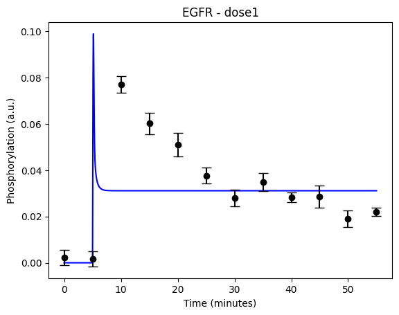
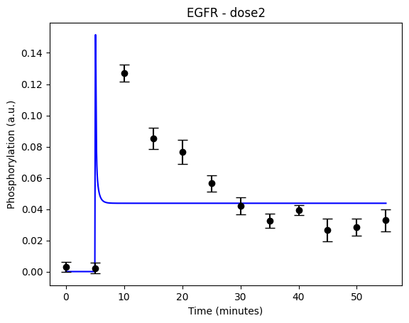
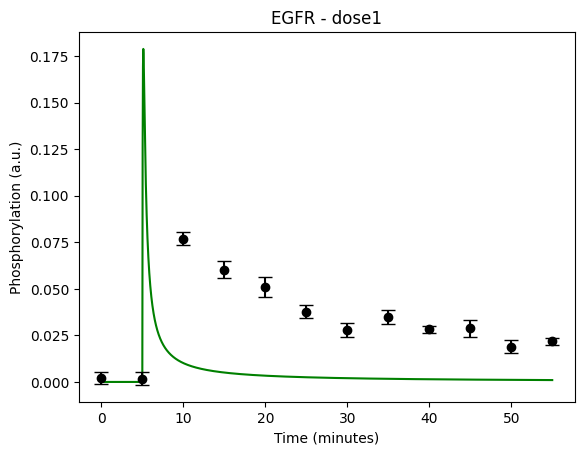
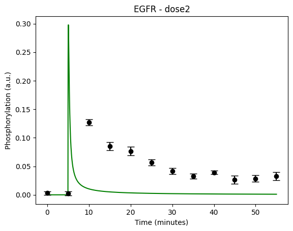
During the following exercises you will take on the role of a system biologist working in collaboration with an experimental group. The experimental group is focusing on the cellular response to growth factors, like the epidermal growth factor (EGF), and their role in cancer. The group have a particular interest in the phosphorylation of the receptor tyrosine kinase EGFR in response to EGF and therefore perform an experiment to elucidate the role of EGFR. In the experiment, they stimulate a cancer cell line with EGFR and use an antibody to measure the tyrosine phosphorylation at site 992, which is known to be involved in downstream growth signalling. The data from these experiments show an interesting dynamic behavior with a fast increase in phosphorylation followed by a decrease down to a steady state level which is higher than before stimulation (Figure 1). Figure 2 showcases a similar behavior in response to a stronger stimulation.

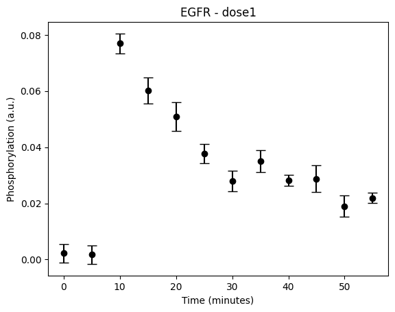
Figure 1: The experimental data. A cancer cell line is stimulated with EGF at time point 5, and the response at EGFR-pY992 is measured

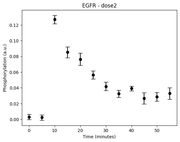
Figure 2: The experimental data. A cancer cell line is stimulated with EGF at time point 5, and the response at EGFR-pY992 is measured

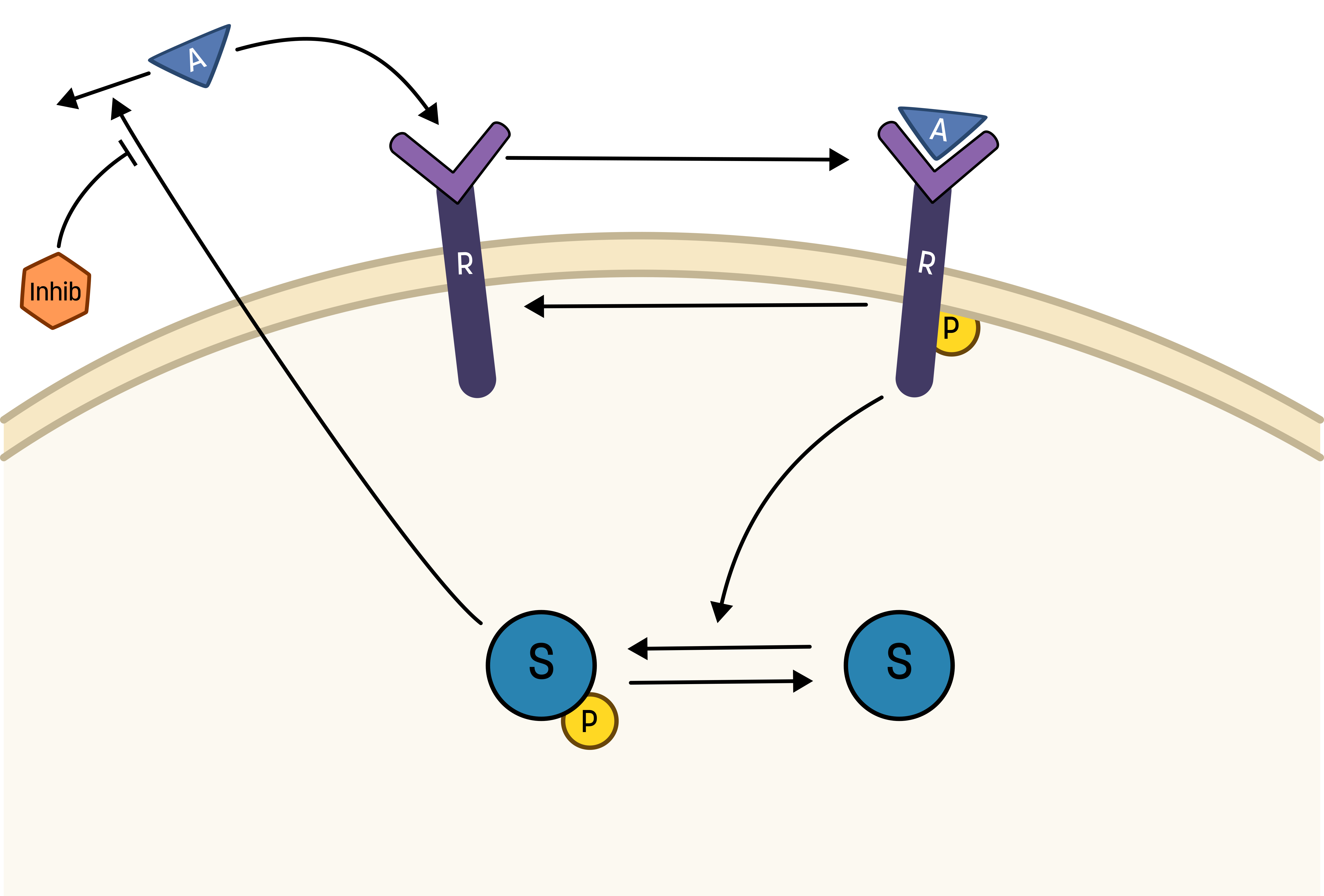
The experimental group does not know the underlying mechanisms that give rise to this dynamic behavior. However, they have two different ideas of possible mechanisms, which we will formulate as hypotheses below. The first idea is that there is a negative feedback transmitted from EGFR to a downstream signalling molecule that is involved in dephosphorylation of EGFR. The second idea is that a downstream signalling molecule is secreted to the surrounding medium and there catalyses breakdown of EGF, which also would reduce the phosphorylation of EGFR. The experimental group would like to know if any of these ideas agree with their data, and if so, how to design experiments to find out which is the more likely idea. To generalize this problem, we refer to EGF as the Activator (A), and EGFR as Receptor (R)

Create a Python script and import the necessary packages

Start by creating a file that ends in .py, for example main.py or main.ipynb if you prefer to work in notebooks, and open it in your favorite text editor (if you do not have a favorit editor yet use VS Code).

We need to import some packages to get access to functions not available in the standard version of Python. You will need numpy, matplotlib and json to start with.

You can import packages in a few different ways: import ..., from ... import .... To avoid long names you can also use the as statement to give the imported packages a new name: import matplotlib.pyplot as plt

Typically, the imports are done at the top of the script:

# Imports
# to import write either:
# import ...
# import ... as ...
# from ... import ...
import os
import re
import numpy as np
import matplotlib.pyplot as plt
import sund
import json
from scipy.stats import chi2
from scipy.optimize import Bounds
from scipy.optimize import dual_annealing, differential_evolution, shgo, direct, minimize
import sys
import csv
import random
import requests

from json import JSONEncoder
class NumpyArrayEncoder(JSONEncoder):
    def default(self, obj):
        if isinstance(obj, np.ndarray):
            return obj.tolist()
        return JSONEncoder.default(self, obj)

We also give you a predefined class NumpyArrayEncoder that will help you package numpy arrays into .json structures (via converting the arrays to lists using the .tolist() function).

If you haven't already, create a python file, (we will assume it is named python_sund.py) and add the imports listed above to the script.

Download and load the experimental data

Start by downloading the data in either of the following three ways:

A) Manually download, by right-clicking and saving

Right-click on this link, and select "save link as". Put the datafile in your working directory.

B) Using requests in Python

Load the file using a url request and save to a file using the open function and the json.dump function.

r = requests.get('https://isbgroup.eu/edu/assets/Intro/Files/data_2024-03-12.json')

with open('data_2024-03-12.json', 'w') as f:
    json.dump(r.json(),f)

C) Using the system function curl (note - this might be troublesome on Windows computers)

Use your operating system terminal to download the data using curl. Notice, that the code below will put the data in your current location, so make sure that you are in the working directory.

curl "https://isbgroup.eu/edu/assets/Intro/Files/data_2024-03-12.json" > data_2024-03-12.json

Next, you will need to load the experimental data into Python. You will need to open the file with the open function and then using the json.load function to load the data. To avoid having to manually close the file and adapt to errors, the best practise is to use the with statement.

with open("data_2024-03-12.json", "r") as f:
    data = json.load(f)

Now, observe the data using print().

print(data)

The data structure is a dictionary, the fields in the dictionary are arrays. You can get the keys of the dictionary with data.keys() and access the data fields with data["key_name"]. Remember, you can read more about a function or object with the command help(function/object) or to an object's attribute you can also use dir(object). To get access to help/dir you need to launch the Python REPL by typing python into to your terminal.

The data downloaded consists of three datasets: dose1, dose2, and step_dose. We will use dose1 and dose2 for estimating the model parameters, and the step_dose for model validation. However, to do this in an code efficient way, we will need to put step_dose in its own dictionary

Split the data into estimation and validation data

To move the step_dose data to its own dictionary, we can simply use the dictionary function pop() which removes the field from data and stores it in our new dictionary data_validation.

data_validation = {}
data_validation['step_dose'] = data.pop('step_dose')

Implement and then call the plot_data function

As we have more than one dataset in our estimation data, we will always want to plot both of these data sets. Implement a plot_dataset function that can plot one of the datasets. The function can be placed either at the top of the script (after the imports) or before it is used, the exact location does not matter in Python. The function should take data as input and plot all the points, with error bars. It should have nice labels and a title.

Useful Python/matplotlib commands (remember that we renamed matplotlib.pyplot as plt): plt.errorbar, plt.xlabel, plt.ylabel, plt.title, plt.plot.

def plot_dataset(data, face_color='k'):
    plt.errorbar(data['time'], data['mean'], data['SEM'], linestyle='None', marker='o', markerfacecolor=face_color, color='k', capsize=5)
    # add nice x- and y-labels

Next, we want to create a function which can plot multiple datasets. A good way of doing this in a generalized way is by calling plot_dataset() from another function wrapping function that gives plot_dataset() the correct data, in this way we can reuse plot_dataset() to plot any data. Lets us call this overarching function plot_data().

def plot_data(data, face_color='k'):
    for experiment in data:
        plt.figure()
        plot_dataset(data[experiment], face_color=face_color)
        plt.title(f'EGFR - {experiment}')

Here, we loop over the fields in data and give plot_dataset() the data of the different doses. We get different figures using plt.figure(). Lastly, using f-strings, we can make a nice title that includes the field name from the data structure. F-strings allows us to include variables in strings if wrapped with {}, in this case {experiment}.

To make the plot visible, we sometimes have to run plt.show(). This will display all plots generated, and pause the python script until the plots are closed. Therefore, it might be a good idea to keep the plt.show() at the end of your script.

Plot the data and and make sure your plots look nice.

plot_data(data)
plt.show()

Remember to give the axes labels.

You should now have a plot of the data. You can self-check if you have implemented things using the box below.

(spoilers) Self-check: Have you plotted the data correctly?

If you have implemented everything correctly, your plot should look something like the figures below.

Furthermore, your code should look something like this.

Code sync

# Import packages
import os
import re
import numpy as np
import matplotlib.pyplot as plt
import sund
import json
from scipy.stats import chi2
from scipy.optimize import differential_evolution, dual_annealing, shgo, direct, minimize
import sys
import csv
import random

from json import JSONEncoder
class NumpyArrayEncoder(JSONEncoder):
    def default(self, obj):
        if isinstance(obj, np.ndarray):
            return obj.tolist()
        return JSONEncoder.default(self, obj)

# Download the experimental data:
r = requests.get('https://isbgroup.eu/edu/assets/Intro/Files/data_2024-03-12.json')

with open('data_2024-03-12.json', 'w') as f:
    json.dump(r.json(),f)

# Load and print the data
with open("data.json", "r") as f:
    data = json.load(f)

print(data)

# split the data into training and validation data
data_validation = {}
data_validation['step_dose'] = data.pop('step_dose')

print(data_validation)

# Define a function to plot one dataset
def plot_dataset(data, face_color='k'):
    plt.errorbar(data['time'], data['mean'], data['SEM'], linestyle='None', marker='o', markerfacecolor=face_color, color='k', capsize=5)
    plt.xlabel('Time (minutes)')
    plt.ylabel('Phosphorylation (a.u.)')


# Define a function to plot all datasets
def plot_data(data):
for experiment in data:
    plt.figure()
    plot_dataset(data[experiment])
    plt.title(f'EGFR - {experiment}')


plot_data(data)

plt.show()

Define, simulate and plot a first model

The experimentalists have an idea of how they think the biological system they have studied works. We will now create a mathematical representation of this hypothesis.

About the hypothesis

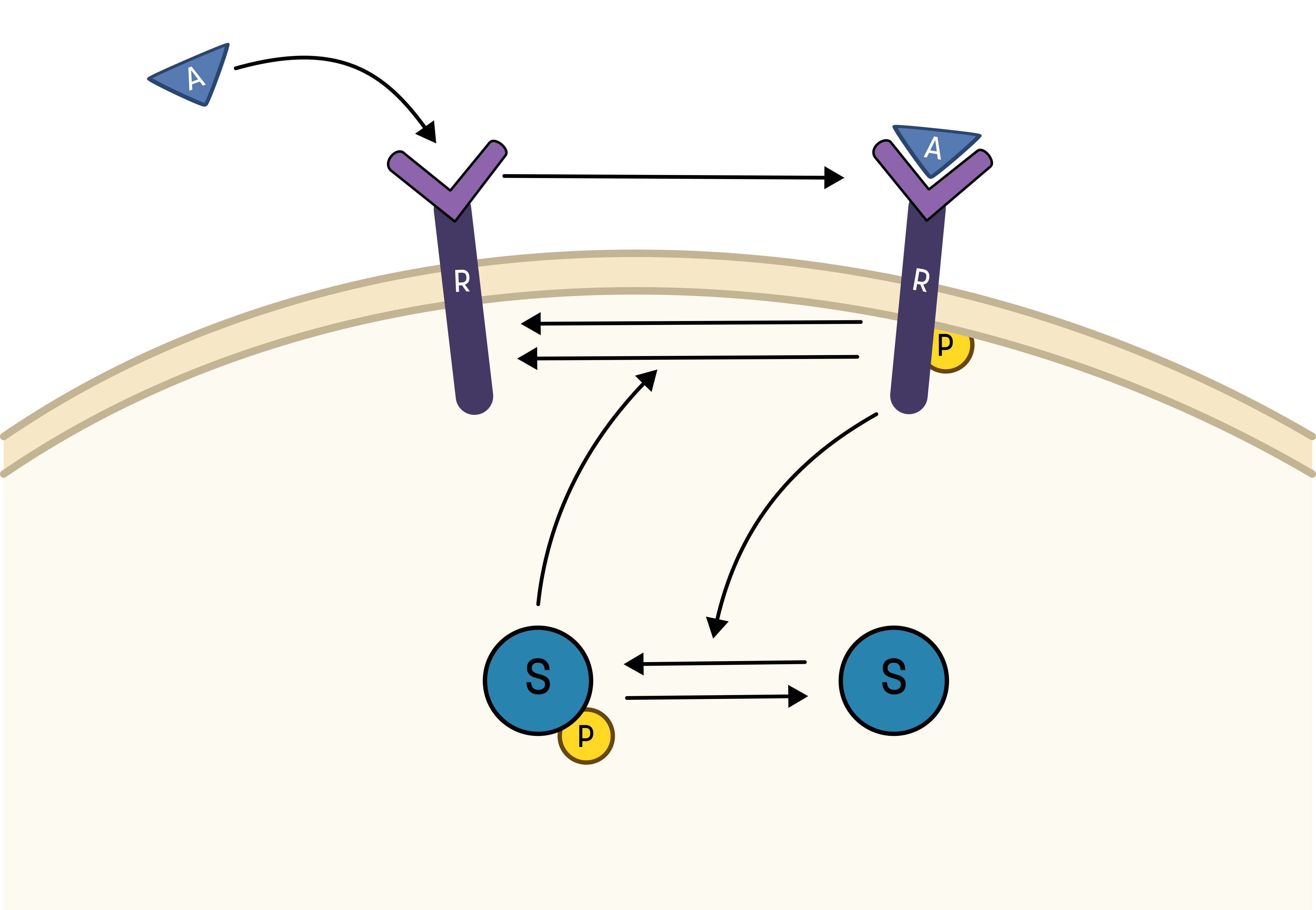
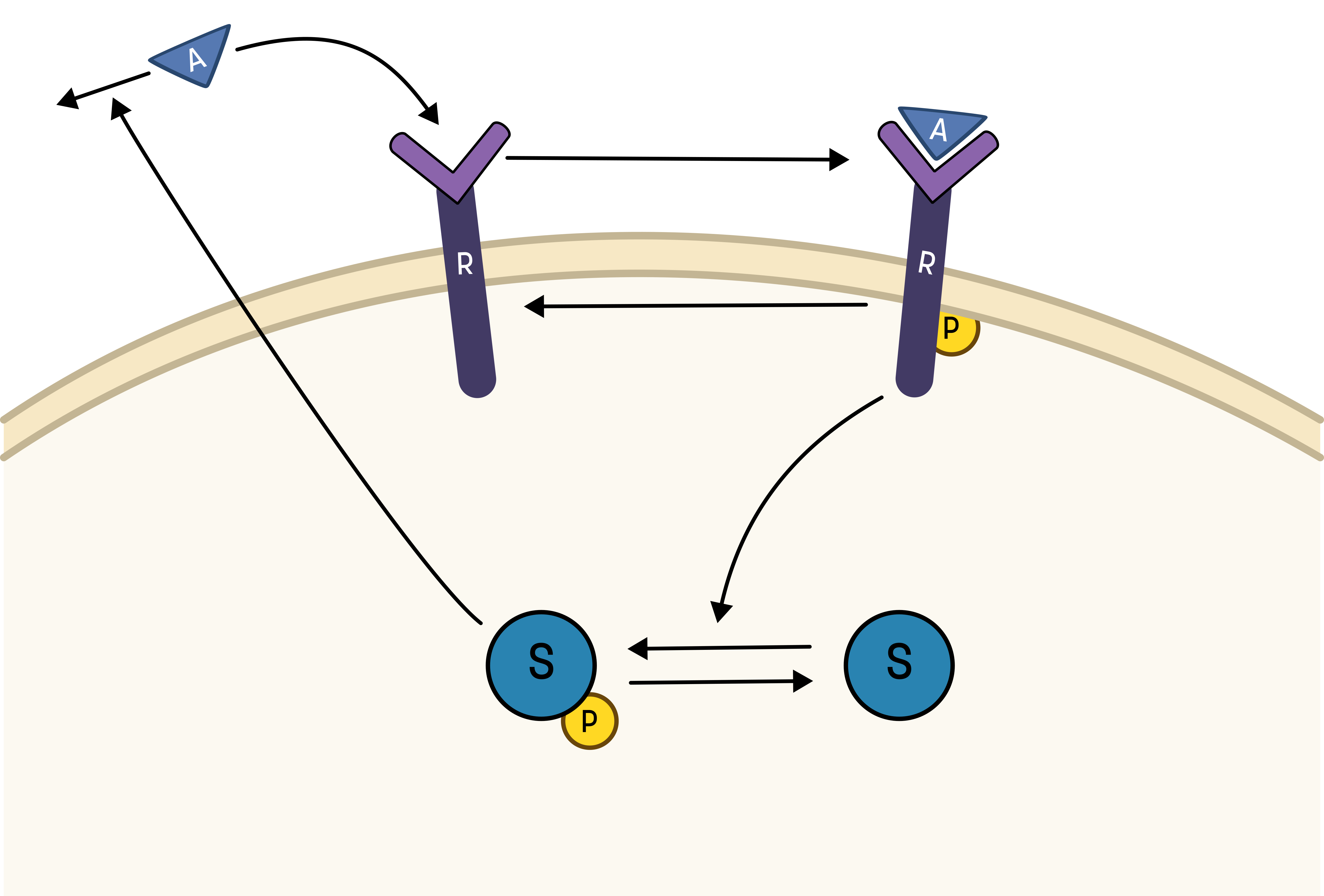
To go from the first idea to formulate a hypothesis, we include what we know from the biological system:

• A receptor (R) is phosphorylated (Rp) in response to a stimulation (A)
• A downstream signalling molecule (S) is activated as an effect of the phosphorylation of the receptor
• The active downstream signalling molecule (Sp) is involved in the dephosphorylation of the receptor
• Phosphorylated/active molecules can return to inactive states without stimuli

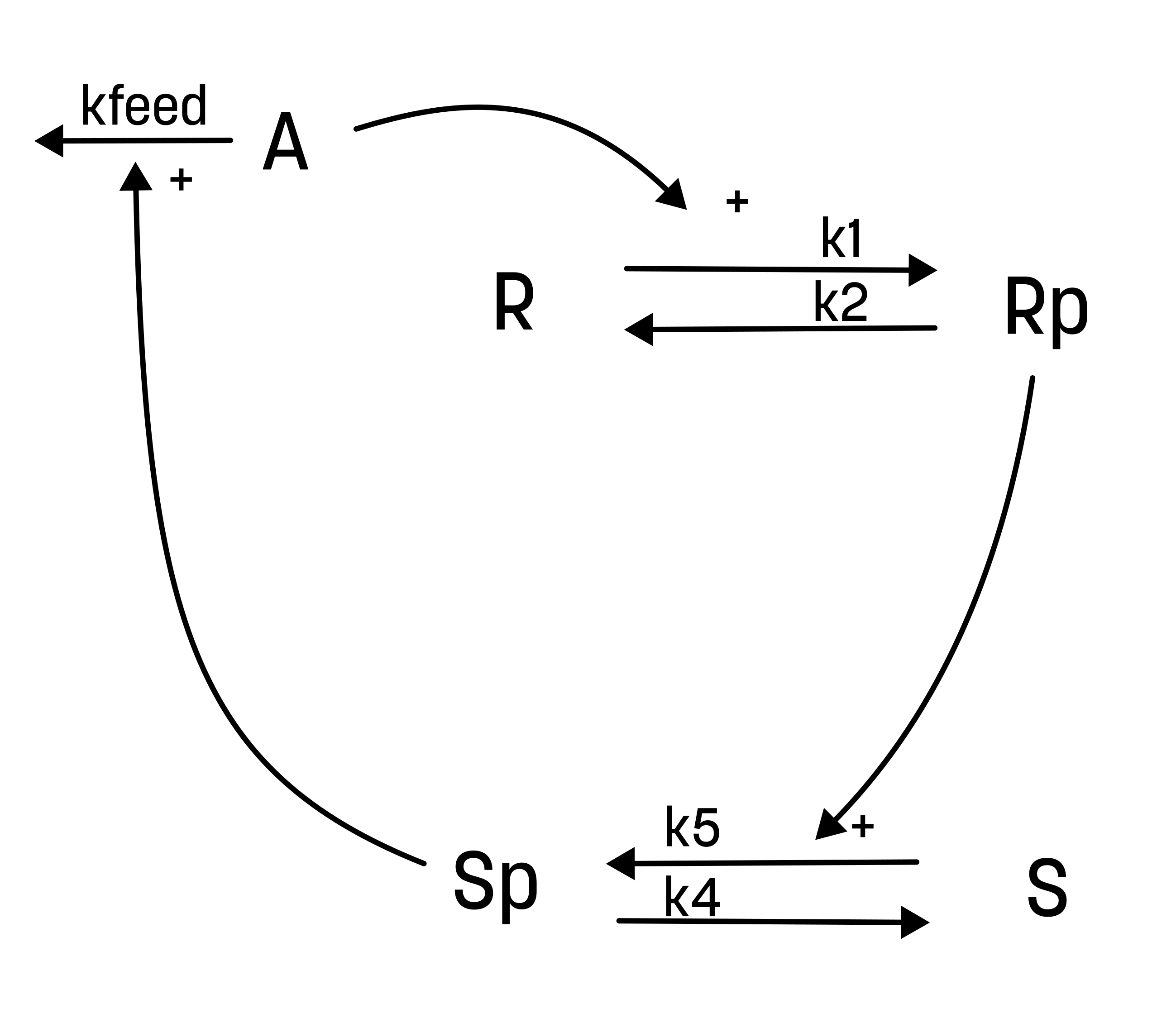
Based on the behavior in the data, and the prior knowledge of the system, the experimentalists have constructed the hypothesis depicted in the figure below.

From this hypothesis, we can draw an interaction graph, along with a description of the reactions.

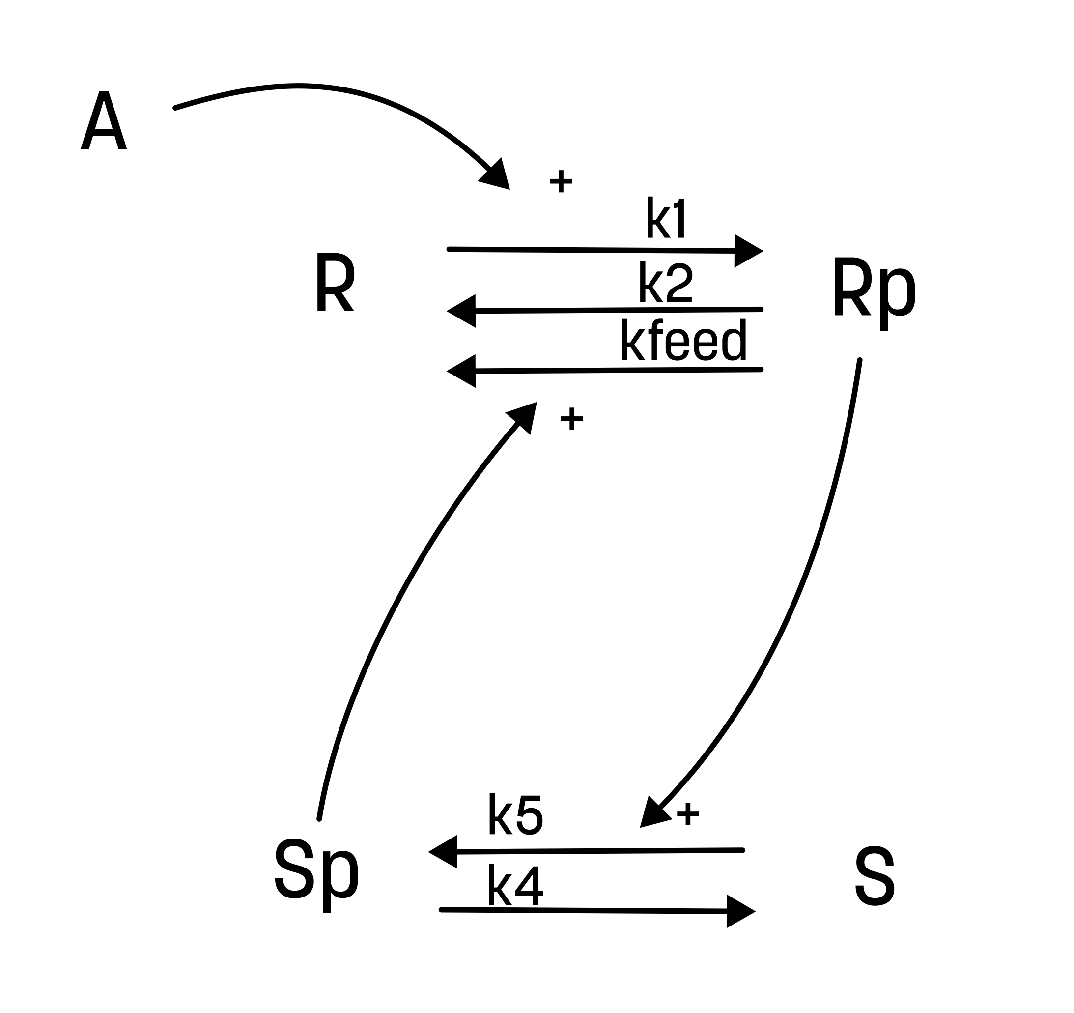
The reactions are as follows:

• Reaction 1 is the phosphorylation of the receptor (R). It depends on the state R, with the input A and the parameter k1.
• Reaction 2 is the basal dephosphorylation of Rp to R. It depends on the state Rp with the parameter k2.
• Reaction 3 is the feedback-induced dephosphorylation of Rp to R exerted by Sp. This reaction depends on the states Rp and Sp with the parameter kfeed.
• Reaction 4 is the basal dephosphorylation of Sp to S. It depends on the state Sp with the parameter k4.
• Reaction 5 is the phosphorylation of S to Sp. This phosphorylation is regulated by Rp. The reaction depends on the states S and Rp, with the parameter k5.

Rp is what have been measured experimentally.

The experimentalist have guessed the values of both the initial conditions and the parameter values

Initial values	Parameter values
R(0) = 1	k1 = 1
Rp(0) = 0	k2 = 0.0001
S(0) = 1	kfeed = 1000000
Sp(0) = 0	k4 = 1
	k5 = 0.01

The next step now is to implement the hypothesis as a mathematical model, and then simulate the model using the SUND package.

About the SUND package and object-oriented programming

The SUND package for implementing and simulating ordinary differential equation (ODE) and differential algebraic equation (DAE) models, uses an object-oriented approach. In object-oriented programming, we work with objects which can have internal values and functions. In the case of a model, such a model object will contain e.g. equations, time unit, and parameter values.

Furthermore, an object is created from a generic "template" referred to as a class. In the case of a model, we could create different model objects from the same model class. For example, if we have a model for meal consumption on a whole-body level for a generic person, we can use the model class to create custom model objects for specific individuals with e.g. different weight, height or age.

Moreover, the sund package also uses objects for simulation. The simulation object takes model objects as input, as well as a definition of what to simulate with e.g. specific time points. We use the function Simulate of the simulation object to run the simulation. Note that the simulation object then retains the values (such as the state values) after the simulation.

In summary, we start by creating a model class, which we use to create model objects, which are then used to create simulation object. As a final note, classes are typically named using CamelCase, and objects using snake_case in Python. Now, we will implement the first model, and go through the steps of creating the classes and objects.

You can find more details about the sund package in the documentation.

Implement the hypothesis as a mathematical model

We will now go through the steps on how to implement the hypothesis as a mathematical model

Defining the model equations

First, we must define the mathematical model in a format that the SUND toolbox understands. Start by creating a text file (the code in these instructions assumes the name M1.txt. If you name your file something else you need to account for this in your code), and use the following model formulation as a template. Update it to include all equations needed for the hypothesis. The VARIABLES heading contain the reaction rates.

To define the model output (measurement equation), we define use the FEATURES heading.

Note that the text file must contain all headers below (beginning with ##########)

########## NAME
// Comments are made with '//'
M1
########## METADATA
timeunit = m
########## MACROS
########## STATES
ddt_R = r2-r1 // You can also write d/dt(R) = ... if you prefer
ddt_Rp = r1-r2
ddt_S = 0 // remember to update
ddt_Sp = 0 // remember to update

R(0) = 1
Rp(0) = 0
S(0) = 1
Sp(0) = 0
########## PARAMETERS
k1 = 1
k2 = 0.0001
########## VARIABLES
r1 = R*A*k1
r2 = Rp*k2
########## FUNCTIONS
########## EVENTS
########## OUTPUTS
########## INPUTS
A = A_in @ 0 // @ 0 means that A has the value 0 if A_in is not given as input
########## FEATURES
y_sim = Rp

Known bug: Step response inputs and integration issues

We need to add an event that internally resets the simulation when the input change happens. For this model, we can add two events which trigger when the A input changes value (A > 0 and A <= 0). Add the following under the EVENTS header:

event1 = A>0
event2 = A<=0 

Install the model

To install your model so that it can be used by Python, you use the SUND package function installModel("filename"). This will basically define a new model class which contains the mathematical model. This class can then be imported and used to create model objects. Now, install the model.

# Install the model by using the sund function 'installModel'
# To verify that the model has been installed try running 'installedModels' afterwards
sund.installModel('M1.txt')
print(sund.installedModels())

Import the model class

Once a model has been installed it can be imported to Python. To do this use the sund function importModel(modelname) (with the model name given in the model file). The function will return a model class which should be stored in variable, say M1.

# Import the model by using the sund function 'importModel'
# The function return the model class which should be stored in variable, say 'M1'
M1 = sund.importModel("M1")

Reinstalling a model that has already been imported

If the model has already been imported, Python must be restarted before (re)installing the model. This is mostly an issue if running the model from within a notebook. In that case, you must restart the kernel before restarting the model.

Create a model object from the model class

To create a model object from the M1 model class, call the class constructor as follows:

m1 = M1()

A new model object is now stored in the variable m1.

Note that the parameter and state values of the model object defaults to what was written in the model file when it was installed. This means that if you change the values in the text file without reinstalling the model, nothing will happen.

You can give custom values using the parametervalues and statevalues keywords when creating the model object, or by setting the corresponding attributes (.parametervalues) of the model object after it as been constructed. To reset the values of the model object to the values from the model class, use the .ResetParameters() function of the model object. You can reset the state values using the .ResetStatesDerivatives() function.

Also note that initial conditions for derivatives are needed for DAE:s (differential algebraic equations) when specifying state values, but are not for ODE:s (ordinary differential equations).

Try to change the parameter/state values, and then reset the values. E.g. like this:

m1.statevalues = [2, 2, 2, 2]
print(m1.statevalues)
m1.ResetStatesDerivatives()
print(m1.statevalues)

Create an activity object

In the model file, we defined the given inputs to the model. These inputs can either be outputs from other models, or from an activity object. Here, the model needs an input "A_in", which we will now give as an output from a custom activity object.

Note that an activity can have multiple outputs, which are added to the activity object by using the .AddOutput function:

# Create an activity object, which sets A_in to 1 at t=5. 

activity = sund.Activity(timeunit='m')
activity.AddOutput(sund.PIECEWISE_CONSTANT, "A_in", tvalues = [5], fvalues=[0,1])

You can find more information on the acitivty object here.

Using the data file

As we have included the stimulation details in the experimental data file you downloaded, one can use the details in the input field to define the activity instead of writing them manually.

activity = sund.Activity(timeunit='m')
activity.AddOutput(sund.PIECEWISE_CONSTANT, "A_in", tvalues = data['dose1']['input']['A_in']['t'], fvalues=data['dose1']['input']['A_in']['f'])

Create a simulation object and simulate

The simulation of models is carried out by a simulation object, which can include one or more model objects, and (optionally) one or more activity object. If you want to use multiple models/activitiy objects, put them in a list (e.g. [m1a, m1b]).

To create a simulation object, call the class constructor Simulation from the SUND package. You will need to provide the model objects that should be included when you do the constructor call.

# Create two new Simulation object for the m1 object using the constructor `sund.Simulation(models=models)` from the sund package and assign the two different stimulation activities corresponding to the training data.
m1_simulation = sund.Simulation(models = m1, activities= activity,  timeunit = 'm')

The simulation object has a function Simulate which can be used to perform a simulation. To use this, you need to give the simulation object: time points to simulate (a list of points), and the unit of the time points ('s' for seconds, 'm' for minutes, 'h' for hours). This can be done in three different ways:

1. set the timevector and timeunit attributes of the simulation object,
2. use the timevector and timeunit keywords when creating the Simulation, or
3. use the keywords when running the simulation using Simulate.

using the timeunit keyword

Notice: if you use the timeunit keyword for the .Simulate function, you will update the time unit of simulation object, not just for the current simulation. Therefore, it is not recommended to do this. Instead, to be clearer, set the timeunit of the Simulation object before simulating.

Now, create a simulation of either of the experiments. If you don't remeber the name of the experiment, you can print them using print(f"experiments: {data.keys()}")

# Simulate the m1_simulation object, for any of the experiments, remember to specify the time vector ([times to simulate]) and timeunit ('s' | 'm' | 'h' ). 
timepoints = np.arange(0, data[experiment]['input']['A_in']['t'][-1]+0.01, 0.01) # Time points between 0 and 55, with a steplength of 0.01.
m1_simulation.Simulate(timevector=timepoints)

About the default parameter values

Note that the default values of the states/parameters in the simulation object will be set to the values of the model objects that was used to create the simulation object. As when creating the model objects, you can also specify custom values for the simulation object using the parametervalues and statevalues keywords/attributes. The ResetParameters() and ResetStatesDerivatives() functions will reset the values to the current values of the model object (note that if the model model object has been updated the simulation object will be not be reset to the original values).

About using multiple models in the simulation

If you are using multiple model objects to create the simulation objects, these can be connected by using the ########## OUTPUTS and ########## INPUTS cells within the models. For example, the output of one model can be used as the input to another model.

After you have simulated the m1_simulation object, the object will be updated. The statevalues now correspond to the final point in the simulation, but more importantly we now have the simulated values of the measurements defined as features.

Observe the simulation result

The simulation object will store the simulation result for every feature specified in the model file/files, i.e. everything specified under the ########## FEATURES cell. The result is stored in an attribute called featuredata where each column represent one feature, thus the first feature can be accessed using featuredata[:,0]. You can get the feature names using the attribute featurenames.

Print and/or plot the simulation result of the feature y_sim for the times simulated above as you did before. Does it look like you would expect? As mentioned, the state values are updated in the simulation object, so what happens if you run the simulation twice?

# Print the result of the simulation above
print(f"Values after first simulation: {m1_simulation.featuredata[:,0]}")
print(f"featurenames: {m1_simulation.featurenames}")

# Also try to simulate twice, before plotting, does it change the values? 
m1_simulation.Simulate(timevector=timepoints)
print(f"Values after simulating twice: {m1_simulation.featuredata[:,0]}")

Observe states and derivatives

If you take a look at the states and derivatives of the simulation object, using the attribute statevalues and derivativevalues, you will see that they have new values after running the simulation, different from the initial values provided in the model object. This is intentional, the simulation will keep the updates states/derivatives values so that another simulation can continue where the previous one stopped. Note however, that the states and derivatives of the model object m1 are not automatically updated to the simulation new states and derivatives. The idea is that the model objects should store the desired initial condition, such that any new simulation will start from the correct state. The states/derivatives of a simulation object can be reset to the states/derivatives of those in the model objects by calling the function ResetStatesDerivatives(). This allows simulation to start with the original configurations. The states/derivatives of the model objects in a simulation can also be updated to the new states/derivatives of the simulation by calling the function UpdateModelObjects().

Now, print the state values, then reset the states/derivatives using ResetStatesDerivatives() and print the values again. Note that they differ (if you have simulated at least once).

# Observe the states values of both the simulations object 'm1_simulation'
# and the model object 'm1'. Note that they differ. 
print(f"Simulation state values before reset: {m1_simulation.statevalues}")
print(f"Model state values before reset: {m1.statevalues}")

# Reset the states of the simulation object, and check the state values again.
m1_simulation.ResetStatesDerivatives()
print(f"Simulation state values after reset: {m1_simulation.statevalues}")
print(f"Model state values after reset: {m1.statevalues}")

Running the same simulation with different parameter values

What we most often want to do is to change the values of the parameters, but keep the initial state values the same. We can use the simulation object to do this, by running two simulations with different values of the parameters, and by resetting the state values. Both these things can be done in the call to the Simulate function by using the parametervalues and resetstatesderivatives keywords.

Do two simulations, with different parameter values but with the same initial conditions. Print and/or plot the results. Does it behave as you expect?

# Run two simulations with different parameter values, but the same initial conditions. 
m1_simulation.Simulate(parametervalues=[1, 0.0001, 1000000, 1, 0.01], resetstatesderivatives=True)
print(f"Simulation state values with first parameter set: {m1_simulation.statevalues}")

m1_simulation.Simulate(parametervalues=[1, 1, 100, 1, 1], resetstatesderivatives=True)
print(f"Simulation state values with first parameter set: {m1_simulation.statevalues}")

Simulate the hypothesis using the provided parameter values, plot and compare to data

Since we have two datasets, collected with different stimulation strength, we need to construct two simulation objects with different activities corresponding to the data stimulation. To keep track of the simulations, a good approach is to keep them in a dictionary. Create the two simulation objects, and store them in a dictionary. You need to first create two activity objects, and then create the simulation objects. Use the dose values from the data. Remember to set the timeunit of the simulation to minutes.

m1_sims = {} # Create an empty dictionary

m1_sims['dose1'] = sund.Simulation(...) # update with activity 1
m1_sims['dose2'] = sund.Simulation(...) # update with activity 2

We start by defining a function that takes the parameter values, simulation object, and timepoints as input, and plots the simulation. We also include the color (color='b') and feature to plot (y_sim) with default arguments, this allow us to reuse the same function even if we need to change them latter.

# Define a function to plot the simulation
def plot_sim(params, sim, timepoints, color='b', feature_to_plot='y_sim'):
    # Setup, simulate, and plot the model
    sim.Simulate(timevector = timepoints,
                    parametervalues = params,
                    resetstatesderivatives = True)

    feature_idx = sim.featurenames.index(feature_to_plot)
    plt.plot(sim.timevector, sim.featuredata[:,feature_idx], color)

Following, we now combine our plot_sim and plot_dataset functions to create a function that plots the simulation and data togheter in a generalized way, making use of the strucutre that we set up the data and simulations with.

# Define a function to plot the simulations together with the data
def plot_sim_with_data(params, sims, data, color='b'):

    for experiment in data:
        plt.figure()
        timepoints = np.arange(0, data[experiment]["time"][-1]+0.01, 0.01)
        plot_sim(params, sims[experiment], timepoints, color)
        plot_dataset(data[experiment])
        plt.title(f'EGFR - {experiment}')

As you might notice, we utilize the experiment to seperate the simulation and data for the different activities, as we loop over the fields in data.

Finally, we use the newly defined funtion to plot both the model simulation and data.

params0_M1 = [1, 0.0001, 1000000, 1, 0.01] # = [k1, k2, kfeed, k4, k5]
plot_sim_with_data(params0_M1, m1_sims, data)

(spoilers) Self-check: Have I implemented the model/code correctly?

If you have done everything correctly, you should have two figures which looks like this for the first hypothesis with the given values:

The code should now look something like what is in the box below:

Code sync

#(all code from last sync)

# Install the model
sund.installModel('M1.txt')
print(sund.installedModels())

# Import the model class and create a model object
M1_class = sund.importModel("M1")
m1 = M1_class() # Create a model object from the model class

# Create a simulation object
m1_simulation = sund.Simulation(models = m1, activities = activity, timeunit = 'm')

# Create activities for the doses in data
activity1 = sund.Activity(timeunit='m')
activity1.AddOutput(sund.PIECEWISE_CONSTANT, "A_in", tvalues = data['dose1']['input']['A_in']['t'], fvalues=data['dose1']['input']['A_in']['f'])

activity2 = sund.Activity(timeunit='m')
activity2.AddOutput(sund.PIECEWISE_CONSTANT, "A_in", tvalues = data['dose2']['input']['A_in']['t'], fvalues=data['dose2']['input']['A_in']['f']) 

# Add your simulation objects into a dictionary 
m1_sims = {}
m1_simulations['dose1'] = sund.Simulation(models = m1, activities = activity1, timeunit = 'm')
m1_simulations['dose2'] = sund.Simulation(models = m1, activities = activity2, timeunit = 'm')

# Define a function to plot the simulation
def plot_sim(params, sim, timepoints, color='b', feature_to_plot='y_sim'):
    # Setup, simulate, and plot the model
    sim.Simulate(timevector = timepoints,
                    parametervalues = params,
                    resetstatesderivatives = True)

    feature_idx = sim.featurenames.index(feature_to_plot)
    plt.plot(sim.timevector, sim.featuredata[:,feature_idx], color)


# Define a function to plot the simulations together with the data
def plot_sim_with_data(params, sims, data, color='b'):

    for experiment in data:
        plt.figure()
        timepoints = np.arange(0, data[experiment]["time"][-1]+0.01, 0.01)
        plot_sim(params, sims[experiment], timepoints, color)
        plot_dataset(data[experiment])
        plt.title(f'EGFR - {experiment}')


# Plot the model with the given parameter values:
params0_M1 = [1, 0.0001, 1000000, 1, 0.01] # = [k1, k2, kfeed, k4, k5]
plot_sim_with_data(params0_M1, m1_simulations, data)

Improving the agreement manually (if there is time)

If you have extra time, try to find a combination of parameter values that improves the agreement to data by manually changing the parameter values.

Checkpoint and reflection

This marks the end of the first section of the exercise. Show your figure which shows how well the model agrees with the data.

Questions to reflect over

• Why do we simulate with a time-resolution higher than the resolution of the data points?
• When is the agreement good enough?
• What could be possible reasons why not all states of the model are measured experimentally?
• (optional) Was it easy finding a better agreement? What if it was a more complex model, or if there were more data series?

---

Evaluating and improving the agreement to data

Clearly, the agreement to data (for the given parameter set) is not perfect. A question now arises: how good does the model simulation agree with data? We typically evaluate this using a cost function

About the cost function

We typically evaluate the model agreement using a sum or squared residuals, weighted with the uncertainty of the data, often referred to as the cost of the model agreement.

\[v\left(\theta\right)=\ \sum_{\forall t}\left(\frac{{y_t -\ {\hat{y}}_t\left(\theta\right)}}{{SEM}_t}\right)^2\]

where \(v(\theta)\) is the cost given a set of parameters \(\theta\), \(y_t\) and \(SEM_t\) is experimental data (mean and SEM) at time \(t\), and \({\hat{y}}_t\) is model simulation at time \(t\). Here, \(y_t-\ {\hat{y}}_t\left(\theta\right)\), is commonly referred to as residuals, and represent the difference between the simulation and the data in each timepoint.

Implement a cost function

Define a function fcost(params, simulation, data) that simulates your model for a set of parameters and returns the cost

Call the simulation's Simulate-function from inside the fcost function to get the simulated values. Remember that we need to reset the state values before starting the simulation.

Calculate the cost using the weighted sum of squares. We use numpy (which we imported as np) functions so sum and weight the residuals.

Since we have two datasets we want to evaluate the model against, we need to do two simulations and add the costs together. First, lets go through an explicit version, and then we go through the more generalizable version you should use

# Explicit version (you should not use this)
def fcost(params, sims, data):

    cost = 0

    sims["dose1"].Simulate(timevector = data["dose1"]["time"], 
                        parametervalues = params,
                        resetstatesderivatives = True)

    y_sim_1 = sims["dose1"].featuredata[:,0]
    y_1 = data["dose1"]["mean"]
    SEM_1 = data["dose1"]["SEM"]

    cost += np.sum(np.square(((y_sim_1 - y_1) / SEM_1)))

    sims["dose2"].Simulate(timevector = data["dose2"]["time"], 
                        parametervalues = params,
                        resetstatesderivatives = True)

    y_sim_2 = sims["dose2"].featuredata[:,0]
    y_2 = data["dose2"]["mean"]
    SEM_2 = data["dose2"]["SEM"]

    cost += np.sum(np.square(((y_sim_2 - y_2) / SEM_2)))

    return cost

As you can notice, we essentially do the same calculations twice. As you can image this scales badly if you have more datasets. A better approach is to make this generalizable.

If you have named your simulations to the same things as in data, you can map simulations to data and iterate over them easily:

# Calculate the cost
def fcost(params, sims, data):

    cost = 0

    for dose in data.keys():
        sims[dose].Simulate(timevector = data[dose]["time"], 
                            parametervalues = params,
                            resetstatesderivatives = True)

        y_sim = sims[dose].featuredata[:,0]
        y = data[dose]["mean"]
        SEM = data[dose]["SEM"]

        cost += np.sum(np.square(((y_sim - y) / SEM)))

    return cost

How to handle 'bad' simulations

A simulation may crash due to numerical errors when solving the differential equations. Often, this is attributed to bad parameter values. To avoid the program crashing due to an error we need to put the Simulation call inside a try/except structure:

def fcost(params, sim, data):
    cost = 0
    for dose in data.keys():
        try:
            sim.Simulate(...)
            ...
            cost += ...
        except Exception as e:
            # print(str(e)) # print exception, not generally useful
            # in-case of exception return a high cost
            cost+= 1e30

Here, the program will try executing everything inside the try-block but if an exception happen it will jump to the except-block.

Calculate the cost of the initial parameter set

Now, let's calculate the cost for the model, given the initial parameter values, using the cost function defined above (fcost). Finally, let's print the cost to the output (by using print and an f-string).

param0_M1 = [1, 0.0001, 1000000, 1, 0.01] # = [k1, k2, kfeed, k4, k5]
cost_M1 =  fcost(param0_M1, m1_sims, data)
print(f"Cost of the M1 model: {cost_M1}")

Test a parameter set which gives a simulation that crashes

In some cases, some parameter sets for some models give numerical issues, typically because the ODEs become very large/small. We can provoke this by simulating with negative parameter values (which you should never do), to test that your cost function handles this situation correctly.

Try to simulate with the parameter set: param_fail = [-1e16, -1e16, -1e16, -1e16, -1e16] and make sure that the cost function handles this. You should expect to get a cost around 1e30 returned. Note that you might get warnings similar to [CVODE WARNING] CVODE Internal t = ..... This is to be expected when you run the failing parameter set.

(spoilers) Self-check: What should the cost for the initial parameter set be if the model is implemented correctly?

The cost for the initial parameter set should be approximately 1652.7.

Code-sync

#(all code from last sync)

# Define and use the cost function
def fcost(params, sims, data):

    cost = 0

    for dose in data.keys():
        try: 
            sims[dose].Simulate(timevector = data[dose]["time"], 
                                parametervalues = params,
                                resetstatesderivatives = True)

            y_sim = sims[dose].featuredata[:,0]
            y = data[dose]["mean"]
            SEM = data[dose]["SEM"]

            cost += np.sum(np.square(((y_sim - y) / SEM)))

        except Exception as e:
            # print(str(e)) # print exception, not generally useful
            # in-case of exception return a high cost
            cost+= 1e30

    return cost

param0_M1 = [1, 0.0001, 1000000, 1, 0.01] # = [k1, k2, kfeed, k4, k5]
cost_M1 =  fcost(param0_M1, m1_sims, data)
print(f"Cost of the M1 model: {cost_M1}")

Evaluating if the agreement is good enough

Now that we have a quantitative measure of how well the model simulation agree with the experimental data, we can evaluate if the agreement is good enough, or if the model should be rejected.

About statistical tests

To get a quantifiable statistical measurement for if the agreement is good enough, or if the model/hypothesis should be rejected, we can use a \(\chi^2\)-test. We compare if the cost is exceeding the threshold set by the \(\chi^2\)-statistic. We typically do this using p = 0.05, and setting the degrees of freedom to the number of residuals summed (i.e. the number of data points).

If the cost exceeds the \(\chi^2\)-limit, we reject the model/hypothesis.

Compare the cost to a \(\chi^2\)-test

We now test if the simulation with the initial parameter sets should be rejected using the \(\chi^2\)-test.

cost = fcost(param0_M1, m1_sims, data)
dgf=0
for experiment in data:
    dgf += np.count_nonzero(np.isfinite(data[experiment]["SEM"]))
chi2_limit = chi2.ppf(0.95, dgf) # Here, 0.95 corresponds to 0.05 significance level
print(f"Chi2 limit: {chi2_limit}")
print(f"Cost > limit (rejected?): {cost_M1>chi2_limit}")

(spoiler) Self-check: Should the model be rejected?

As suspected, the agreement to the data was too bad, and the model thus had to be rejected. However, that is only true for the current values of the parameters. Perhaps this structure of the model can still explain the data good enough with other parameter values? To determine if the model structure (hypothesis) should be rejected, we must determine if the parameter set with the best agreement to data still results in a too bad agreement. If the best parameter set is too bad, no other parameter set can be good enough, and thus we must reject the model/hypothesis.

Code-sync

#(all code from last sync)

# Test if the model with the initial parameter values must be rejected
cost = fcost(params_M1, m1_sims, data)
dgf=0
for experiment in data:
    dgf += np.count_nonzero(np.isfinite(data[experiment]["SEM"]))
chi2_limit = chi2.ppf(0.95, dgf) # Here, 0.95 corresponds to 0.05 significance level
print(f"Chi2 limit: {chi2_limit}")
print(f"Cost > limit (rejected?): {cost_M1>chi2_limit}")

Improving the agreement

Try to change some parameter values to see if you can get a better agreement.

Improve the agreement (manually)

It is typically a good idea to change one parameter at a time to see the effect of changing one parameter. If you did this in the previous section, you can reuse those parameter values.

param_guess_M1 = [1, 0.0001, 1000000, 1, 0.01] # Change the values here and try to find a better agreement, if you tried to find a better agreement visually above, you can copy the values here

cost =  fcost(param_guess_M1, m1_sims, data)
print(f"Cost of the M1 model: {cost}")

dgf=0
for experiment in data:
    dgf += np.count_nonzero(np.isfinite(data[experiment]["SEM"])) 
chi2_limit = chi2.ppf(0.95, dgf)
print(f"Chi2 limit: {chi2_limit}")
print(f"Cost > limit (rejected?): {cost>chi2_limit}")

plot_sim_with_data(param_guess_M1, m1_sims, data)

plt.show()

Improve the agreement using optimization methods

As you have probably noticed, estimating the values of the parameters can be a hard and time-consuming work. To our help, we can use optimization methods. There exists many toolboxes and algorithms (also refered to as optimizers) that can be used for parameter estimation. In this short example, we will use some optimizers from the SciPy toolbox.

Prepare before running the parameter optimization

In its simplest mathematical expression, an optimization problem can look something like this:

\[ \begin{array}{ll} \text{minimize} & v(x) = \text{cost}(x, sims, data) \\ \text{subject to} & \text{lb} \leq x \leq \text{ub}. \end{array} \]

where we minimize the objective function \(v(x)\) which evaluates the parameter values \(x\). The parameter values are constrained to be between the lower bound \(lb\) and the upper bound \(ub\).

The SciPy optimizers follow this general convention, using the following naming:

• func - an objective function (we can use the cost function fcost defined earlier),
• bounds - bounds of the parameter values,
• args - arguments needed for the objective function, in addition to the parameter values, in our case model simulations and data: fcost(param, sims, data)
• x0 - a start guess of the parameter values (e.g. param_guess_M1),
• callback - a "callback" function. The callback function is called at each iteration of the optimization, and can for example be used to save the current solution.
• disp - if the iterations should be printed or not (True/False)

Before you can start to optimize the parameters, we need to setup the required inputs (bounds, start guess and a callback). Since we will use this for most of the algorithms, we can setup these things first.

No guarantee

The optimization problem is not guaranteed to give the optimal solution, only better solutions. Therefore, you might need to restart the optimization a few times (perhaps with different starting guesses) to get a good solution.

Defining the callback fuction

This basic callback function prints the result to the output and also saves the current best solution to a temporary file.

def callback(x, file_name):
    with open(f"./{file_name}.json",'w') as file:
        out = {"x": x}
        json.dump(out,file, cls=NumpyArrayEncoder)

Note that different solvers might have different callback defintitions (e.g. callback(x), callback(x,f,c) or callback(x,f,c)). For this reason, and because we want to give the saved temp files a unique name later, we wrap the callback function with another function.

Setting up the start guess, bounds and necessary extra arguments

The bounds determine how wide the search for the parameter values would be, and the extra arguments are the additional arguments that the cost function needs besides the parameter values (in our case the simulations, and the data)

#param_guess_M1 = [1, 0.0001, 1000000, 1, 0.01] # or the values you found manually
bounds_M1 = Bounds([1e-6]*len(param_guess_M1), [1e6]*len(param_guess_M1)) # Create a bounds object needed for some of the solvers
args_M1 = (m1_sims, data)

Improving the efficency of the optimization by searching in log-space

Due to large differences in parameter bounds, and that in general the bounds are often wide, it is much more efficient to search in log-space, and something you should always do if possible.

In practice, we take the logarithm of the bounds and start guess, and return to linear space before simulating and/or saving the parameter values.

One trick is to wrap the cost function and callback function in another function which handles the transformation before passing the parameter values along to the cost function.

#param_guess_M1 = [1, 0.0001, 1000000, 1, 0.01] # or the values you found manually
args_M1 = (m1_sims, data)
param_guess_M1_log = np.log(param_guess_M1)             
bounds_M1_log = Bounds([np.log(1e-6)]*len(param_guess_M1_log), [np.log(1e6)]*len(param_guess_M1_log)) # Create a bounds object needed for some of the solvers


def fcost_log(params_log, sims, data):
    params = np.exp(params_log.copy())
    return fcost(params, sims, data)

def callback_log(x, file_name='M1-temp'):
    callback(np.exp(x), file_name=file_name)

# res = Optimizatio(...) <--- Here we will run the optimization in the next step 

res['x'] = np.exp(res['x']) # convert back the results from log-scale to linear scale

Running the optimization

Now that we have a cost function, a callback function, and have prepared for searching in log-space, it is time to run the optimization to find better parameter values.

# Setup for running optimization (in log-scale)
#param_guess_M1 = [1, 0.0001, 1000000, 1, 0.01] # or the values you found manually
param_guess_M1_log = np.log(param_guess_M1)     
bounds_M1_log = Bounds([np.log(1e-6)]*len(param_guess_M1_log), [np.log(1e6)]*len(param_guess_M1_log)) # Create a bounds object needed for some of the solvers
args_M1 = (m1_sims, data)

def fcost_log(params_log, sims, data):
    params = np.exp(params_log.copy())
    return fcost(params, sims, data)

def callback_log(x, file_name='M1-temp'):
        callback(np.exp(x), file_name=file_name)

# Setup for the specific optimizer
def callback_M1_evolution_log(x,convergence):
    callback_log(x, file_name='M1-temp-evolution')

res = differential_evolution(func=fcost_log, bounds=bounds_M1_log, args=args_M1, x0=param_guess_M1_log, callback=callback_M1_evolution_log, disp=True) # This is the optimization
res['x'] = np.exp(res['x'])

# Save the result
print(f"\nOptimized parameter values: {res['x']}")
print(f"Optimized cost: {res['fun']}")
print(f"chi2-limit: {chi2_limit}")
print(f"Cost > limit (rejected?): {res['fun']>chi2_limit}")

Computational time for different scales of model sizes

Optimizing model parameters in larger and more complex models, with additional sets of data, will take a longer time that in this exercise. In a "real" project, it likely takes hours if not days to find the best solution.

Saving the optimized parameter values

To avoid overwriting or loosing optimized parameter sets, we save the parameter values to a file, with the model name and cost in the file name.

if res['fun'] < chi2_limit: #Saves the parameter values, if the cost was below the limit. 
    file_name = f"M1 ({res['fun']:.3f}).json"
    with open(file_name,'w') as file:
        json.dump(res, file, cls=NumpyArrayEncoder) #We save the file as a .json file, and for that we have to convert the parameter values that is currently stored as a ndarray into a regular list

Loading previously saved parameter sets

After the optimization, the results is saved into a JSON file.

If you later want to load the parameter set you can do that using the code snippet below. Remember to change file_name.json to the right file name. The loaded file will be a dictionary, where the parameter values can be accessed using res['x']

with open('file_name.json','r') as f: # Remember to update 'file_name' to the right name
    res = json.load(f)

Test different optimizers

As mentioned earlier, scipy offers multiple optimizers. You can see some of them below. As they all are implemented in different ways, they are not equally good at the same problem. We want you to choose some (atleast 2) different optimizers to test and compare how well they perfom.

Differential evolution

# Optimize using differential_evolution
def callback_evolution_M1(x, convergence): # The callback to the differential_evolution optimizer returns both the current point x, and state of convergence
    callback_log(x, file_name='M1-temp-evolution')

result_evolution = differential_evolution(fcost_log, bounds_M1_log, args=args_M1, callback=callback_evolution_M1, disp=True) 

Dual annealing

Dual annealing uses a slightly different callback function. Therefore, we need to define a new one, and keep track of the number of iterations done (niter).

# Optimize using dual annealing
def callback_dual(x,f,c):
    global niter

    if niter%1 == 0:
        print(f"Iter: {niter:4d}, obj:{f:3.6f}", file=sys.stdout)
        callback(np.exp(x), file_name = 'M1-temp-dual.json')
    niter+=1

niter=0
result_dual = dual_annealing(fcost_log, bounds_M1_log, x0=param_guess_M1_log, args=args_M1, callback=callback_dual)

SHGO (simplicial homology global optimization)

SHGO has no display property. It is possible to modify the callback to print the iteration if desired

# Optimize using SHG optimization
def callback_shgo_M1(x):
    global niter
    if niter%1 == 0:
        print(f"Iter: {niter}")
        callback_log(x, file_name='M1-temp-SHGO')
    niter+=1

niter=0
result_shgo = shgo(fcost_log, bounds_M1_log, args=args_M1, callback=callback_shgo_M1, options = {"disp":True})

Direct

# Optimize using DIRECT

def callback_direct(x):
    global niter
    if niter%1 == 0:
        print(f"Iter: {niter}")
        callback_log(x, file_name='M1-temp-DIRECT')
    niter+=1

niter=0
result_direct = direct(fcost_log, bounds_M1_log, args=args_M1, callback=callback_direct)

Minimize

# Optimize using local solvers
method = 'TNC' # 'COBYLA', 'TNC', 'L-BFGS'

def callback_local(x):
    global niter
    if niter%1 == 0:
        print(f"Iter: {niter}")
        callback_log(x, file_name=f'M1-temp-{method}')
    niter+=1

niter=0
result_local = minimize(fcost_log, x0=param_guess_M1_log, method=method, bounds=bounds_M1_log, args=args_M1, callback=callback_local)

Plot and calculate the cost for the best solution found using the optimization

Now, plot the best solution found. Is the agreement good?

The code below will use the results from the latest optimization. However, you can also load a specific parameter set if you want to.

p_opt_M1 = res['x']
plot_sim_with_data(p_opt_M1, m1_sims, data)
print(f"Cost: {fcost(p_opt_M1, m1_sims, data)}")

(spoilers) Self-check: How good solution should I have found?

You should have found a cost that is less than 31. If not, run the optimization a few more times. If you still do not find it, make sure that your model is implemented correctly.

Code sync

# (all code from last sync)

# Improving the agreement manually

param_guess_M1 = [1, 0.0001, 1000000, 1, 0.01] # Change the values here and try to find a better agreement, if you tried to find a better agreement visually above, you can copy the values here

cost =  fcost(param_guess_M1, m1_sims, data)
print(f"Cost of the M1 model: {cost}")

dgf=0
for experiment in data:
    dgf += np.count_nonzero(np.isfinite(data[experiment]["SEM"]))
chi2_limit = chi2.ppf(0.95, dgf)
print(f"Chi2 limit: {chi2_limit}")
print(f"Cost > limit (rejected?): {cost>chi2_limit}")

plot_sim_with_data(param_guess_M1, m1_sims, data)

# Improving the agreement using optimization methods

def callback(x, file_name):
    with open(f"./{file_name}.json",'w') as file:
        out = {"x": x}
        json.dump(out,file, cls=NumpyArrayEncoder)


#param_guess_M1 = [1, 0.0001, 1000000, 1, 0.01] # or the values you found manually
args_M1 = (m1_sims, data)

# Setup for searching in log-scale
param_guess_M1_log = np.log(param_guess_M1)     
bounds_M1_log = Bounds([np.log(1e-6)]*len(param_guess_M1_log), [np.log(1e6)]*len(param_guess_M1_log)) # Create a bounds object needed for some of the solvers

def fcost_log(params_log, sims, data):
    params = np.exp(params_log.copy())
    return fcost(params, sims, data)

def callback_log(x, file_name='M1-temp'):
        callback(np.exp(x), file_name=file_name)

# Setup for the specific optimizer
def callback_M1_evolution_log(x,convergence):
    callback_log(x, file_name='M1-temp-evolution')

res = differential_evolution(func=fcost_log, bounds=bounds_M1_log, args=args_M1, x0=param_guess_M1_log, callback=callback_M1_evolution_log, disp=True) # This is the optimization
res['x'] = np.exp(res['x'])

# Save the result
print(f"\nOptimized parameter values: {res['x']}")
print(f"Optimized cost: {res['fun']}")
print(f"chi2-limit: {chi2_limit}")
print(f"Cost > limit (rejected?): {res['fun']>chi2_limit}")

if res['fun'] < chi2_limit: #Saves the parameter values, if the cost was below the limit. 
    file_name = f"M1 ({res['fun']:.3f}).json"
    with open(file_name,'w') as file:
        json.dump(res, file, cls=NumpyArrayEncoder) #We save the file as a .json file, and for that we have to convert the parameter values that is currently stored as a ndarray into a regular list

# Plot the simulation given the optimized parameters

p_opt_M1 = res['x']
plot_sim_with_data(p_opt_M1, m1_sims, data)

plt.show()

Checkpoint and reflection

Show the plot with the best agreement to data, and the cost for the same parameter set. Do you reject the model? Briefly describe the cost function: What are the residuals? Why do we normalize with the squared uncertainty?

Questions to reflect over

• Why do we want to find the best solution?
• Are we guaranteed to find the best solution?
• Do you reject the first hypothesis?
• If you did not reject the model, how can you test the model further?

---

Prediction based model testing

Estimating the model uncertainty

About how to gather model uncertainty

If the optimization did not encounter big issues you should have been able to find a solution that passed the \(\chi^2\)-test. However, it is still possible that we have not found the right model and/or parameter values. For example, since the data have uncertainty it is possible that we have overfitted to uncertain (incorrect) data. An overfitted model would in general be good at explaining the data used for parameter estimation, but might not be good at explaining new data (i.e. making predictions).

For this reason, we do not only want to find the parameter set with the best agreement to data, but rather all parameter sets that agree with the estimation data. Since collecting all sets of parameter values is infeasible from a computational standpoint, we typically try to find the parameter sets that result in the simulations which gives the extreme (maximal/minimal) simulations in each time point.

The best way of finding the extremes is to directly optimize the value by reformulating the optimization problem, or to use Markov-Chain Monte-Carlo (MCMC) methods. Here, we will not do this due to time-constraints, and will instead use a simple (inferior) approach that simply stores a bunch of parameter sets that result in a cost below the threshold of rejection. This gives us a quick approximation of the uncertainty, which is good enough for this exercise. In future projects, you should try to find the maximal uncertainty.

Create an adapted cost function that also saves acceptable parameter sets

To save all parameters, we need to create a function which both calculates the cost, and stores acceptable parameters. We reuse fcost, and introduce a new variable all_params_M1 to save the acceptable parameter to.

all_params_M1 = [] # Initiate an empty list to store all parameters that are below the chi2 limit
def fcost_uncertainty_M1(param_log, sims, data):

    param = np.exp(param_log) # Assumes we are searching in log-space
    cost = fcost(param, sims, data) # Calculate the cost using fcost

    # Save the parameter set if the cost is below the limit
    if cost < chi2.ppf(0.95, dgf):
        all_params_M1.append(param)
    return cost

Run the optimization a couple of times to get values

Next, we need to run the optimization a couple of times to get some acceptable parameter values.

for i in range(0,5):
    niter = 0
    res = xxx(func=fcost_uncertainty_M1, bounds=bounds_M1_log, args=args_M1, x0=param_guess_M1_log, callback=callback_xxx) # This is the optimization - update for the choosen method

print(f"Number of parameter sets collected: {len(all_params_M1)}") # Prints now many parameter sets that were accepted

Make sure that there are at least 250 saved parameter sets. If you want to, you can save the found parameters to a file:

# Save the accepted parameters to a csv file
with open('all_params_M1.csv', 'w', newline='') as csvfile:
    writer = csv.writer(csvfile, delimiter=',')
    writer.writerows(all_params_M1)

# load the accepted parameters from the csv file
with open('all_params_M1.csv', newline='') as csvfile:
    reader = csv.reader(csvfile, delimiter=',', quoting=csv.QUOTE_NONNUMERIC)
    all_params_M1 = list(reader)

Plot the model uncertainty

To save some time, we randomize the order of the saved parameter sets, and only plot the first 200. Obviously this results in an underestimated simulation uncertainty, but the uncertainty should still be sufficient for this exercise. In a real project, one would simulate all collected parameter sets (or sample using the reformulated optimization problem, or MCMC).

Lets create a function which will shuffle the collected parameter sets, and then plot the selected parameter sets for both of the experimental data.

def plot_uncertainty(all_params, sims, data, color='b', n_params_to_plot=500):
    random.shuffle(all_params)

    for experiment in data:
        # Plot the simulations
        plt.figure() # Create a new figure
        timepoints = np.arange(0, data[experiment]["time"][-1]+0.01, 0.01)

        for param in all_params[:n_params_to_plot]:
            plot_sim(param, sims[experiment], timepoints, color)

        # Plot the data
        plot_dataset(data[experiment])

        plt.title(f'EGFR - {experiment}')

Finally, call the plot_uncertainty function with your collectyed parameter values

plot_uncertainty(all_params_M1, m1_sims, data)

(spoiler) Self-check: Did I implement the prediction correctly?

For the uncertainty step your code should look something like below.

Code sync:

#(all code from previous sync)

# Setup for saving acceptable parameters
all_params_M1 = [] # Initiate an empty list to store all parameters that are below the chi2 limit

def fcost_uncertainty_M1(param_log, model, data):

    cost = fcost_log(params, sims, data)

    # Save the parameter set if the cost is below the limit
    dgf = 0
    for experiment in data:
        dgf += np.count_nonzero(np.isfinite(data[experiment]["SEM"]))

    chi2_limit = chi2.ppf(0.95, dgf) # Here, 0.95 corresponds to 0.05 significance level

    if cost < chi2_limit:
        params_list.append(np.exp(params))

    return cost

# Run the optimization a few times to save some parameters
for i in range(0,5):
    niter = 0
    res = dual_annealing(func=fcost_uncertainty_M1, bounds=bounds_M1, args=args_M1, x0=param_guess_M1_log, callback=callback_dual) # This is the optimization
    param_guess_M1_log = res['x'] # update starting parameters 
print(f"Number of parameter sets collected: {len(all_params_M1)}") # Prints now many parameter sets that were accepted

# Save the accepted parameters to a csv file
with open('all_params_M1.csv', 'w', newline='') as csvfile:
    writer = csv.writer(csvfile, delimiter=',')
    writer.writerows(all_params_M1)

# Plot the uncertainty
plot_uncertainty(all_params_M1, m1_sims, data)

Model validation

Finally, now that we have estimated the model uncertainty, we can validate the model by making predictions of new data with uncertainty.

About the prediction

A prediction can almost be anything, but in practice it is common to use a different input strength (A in the model), or to change the input after a set time. It is also possible to extend the simulated time beyond the measured time points. Finally, it is also possible to use the simulation in between already measured data points.

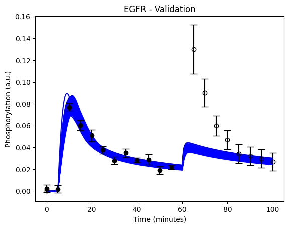
In this case, we will now use the third data set that we excldued earlier data_valdidation. This data is a step response, where A was set to 1 at t = 5 and then A was set to 2 at t = 60.

Plot the validation data

# Test the model against the evaluation experiment
plot_data(data_validation, face_color='w')

Define validation simulation object

First define the new activity corresponding to the validation input.

# define validation activity
activity_validation_M1 = sund.Activity(timeunit='m')
activity_validation_M1.AddOutput(sund.PIECEWISE_CONSTANT, "A_in", tvalues = data_validation['step_dose']['input']['A_in']['t'], fvalues=data_validation['step_dose']['input']['A_in']['f'])

Define a simulation object using this activity.

m1_validation = {}
m1_validation['step_dose'] = sund.Simulation(models = m1, activities = activity_validation_M1, timeunit = 'm')

Plot your prediction, the original data, and the new validation data together

Now, to plot your prediction, the original data, and the new data together, we slightly alter the plot function. Note that we set the facecolor to none for the validation data to more easily differentiate it from the original data.

# Define the plot_sim_with_data function
def plot_validation_with_data(all_params, sims, data_validation, data, color='b', n_params_to_plot=500):

    random.shuffle(all_params)

    for experiment in data_validation:
        plt.figure()
        timepoints = np.arange(0, data_validation[experiment]["time"][-1]+0.01, 0.01)
        for params in all_params[:n_params_to_plot]:
            plot_sim(params, sims[experiment], timepoints, color=color)

        plot_dataset(data_validation[experiment], face_color='w') # Plot the validation data
        plt.title('EGFR - Validation')
    plot_dataset(data['dose1'])    # Since the first part of the validation is the same as for the first dose, we also plot that data

Finally, call the plot_validation_with_data function to plot the validation simulation with data.

plot_validation_with_data(all_params_M1, m1_validation, data_validation, data)

Calculate the cost for the prediction

While we can, most likely, draw conclusions based on the visual agreement, we should also calculate the cost. Calculate the cost for prediction of the data_validation using the best parameter found.

cost_m1_validation = fcost(p_opt_M1, m1_validation, data_validation)

dgf_validation=0
for experiment in data_validation:
    dgf_validation += np.count_nonzero(np.isfinite(data_validation[experiment]["SEM"]))
chi2_limit_validation = chi2.ppf(0.95, dgf_validation)

print(f"Cost (validation): {cost_m1_validation}")
print(f"Chi2 limit: {chi2_limit_validation}")
print(f"Cost > limit (rejected?): {cost_m1_validation>chi2_limit_validation}")

Did your model predict the new data correctly?

(spoiler) Self-check: Did I implement the prediction correctly?

If you did the prediction correctly, you should see something that looks like this:

Code sync:

#(all code from previous sync)

# Plot model prediction with the validation data
def plot_validation_with_data(all_params, sims, data_validation, data, color='b', n_params_to_plot=500):

    random.shuffle(all_params)

    for idx, experiment in enumerate(data_validation):
        plt.figure(1)
        timepoints = np.arange(0, data_validation[experiment]["time"][-1]+0.01, 0.01)
        for params in all_params[:n_params_to_plot]:
            plot_sim(params, sims[experiment], timepoints, color=c)

        plot_dataset(data_validation[experiment], face_color='w') # Plot the validation data
        plt.title('EGFR - Validation')
    plot_dataset(data['dose1'])    # Since the first part of the validation is the same as for the first dose, we also plot that data

plot_validation_with_data(all_params_M1, m1_validation, data_validation, data, color='b')


# Calculate the model agreemnt to the valdidation data
cost_m1_validation = fcost(p_opt_M1, m1_validation, data_validation)

dgf_validation=0
for experiment in data_validation:
    gf_validation += np.count_nonzero(np.isfinite(data_validation[experiment]["SEM"]))
chi2_limit_validation = chi2.ppf(0.95, dgf_validation)

print(f"Cost (validation): {cost_m1_validation}")
print(f"Chi2 limit: {chi2_limit_validation}")
print(f"Cost > limit (rejected?): {cost_m1_validation>chi2_limit_validation}")

Testing an alternative hypothesis

As you should see, the first hypothesis did not predict the new data well. Therefore, you have gone back to the biologists with whom you come up with an alternative second hypothesis: that A is not constant and will instead be removed over time. Implement this alternative hypothesis (given below), check if it can explain the original data, and if it can, collect the uncertainty and check if it can predict the new data correctly.

About the second hypothesis

This hypothesis is similar to the first one, but with some modifications:
1. The feedback-induced dephosphorylation of Rp (reaction 3 in the first hypothesis) is removed. 2. A new feedback-dependent breakdown of the stimulation A is added. This reaction is dependent on the states Sp and A with a parameter kfeed (same name, but a different mode of action).

These differences yield the following interaction-graph:

For the alternative hypothesis, the experimentalist have also guessed the values of both the initial conditions and the parameter values.

Initial values	Parameter values
R(0) = 1	k1 = 5
Rp(0) = 0	k2 = 20
S(0) = 1	kfeed = 10
Sp(0) = 0	k4 = 15
A(0) = 0	k5 = 30

Note that A is now a state and not a constant input.

Start by implementing the new model.

Implement an alternative hypothesis

You have previously implemented and analyzed one hypothesis, now you should do the full analysis also for this second alternative hypothesis. Start by creating a new text file. We assume that you name this model M2.

Since A is now a state, we need to somehow set the value of A when the stimulation is given. To do this, we can use an event. The code block shows how you can set the value of A when the input A_in to the value of A_in (in this case 1).

...

########## EVENTS
input_event = A_in>0, A, A_in
########## OUTPUTS
########## INPUTS
A_in = A_in @ 0

How to set A in the step dose experiment for model 2 (using events)

Note that when making predictions for M2, you will need to set the value of A_in to a value equal to (or smaller than) 0 between the stimulations, otherwise the event cannot trigger a second time. Since we update the value of the state A with the event, the exact time when you set A_in to 0 is not important. Perhaps the easiest way is to create a new activity and simulation object for the M2 prediction, something like this:

activity_validation_M2 = sund.Activity()
activity_validation_M2.AddOutput(sund.PIECEWISE_CONSTANT, "A_in", tvalues = [5, 30, 60], fvalues = [0, 1, 0, 2]) # Set A_in to 1 at t=5, to 0 at t=30 and 2 and t = 60.

Do you reject this model?

(spoilers) Self-check: How can I know if M2 have been implemented correctly?

The cost for the given parameter set should be approximately 2323.8. If it isn't, you might have incorrect equations, or have placed the states or parameters in the incorrect order. It is also possible that you are simulating with parameter values from the wrong model.

Visually, the agreement for the given parameter set should look like this:

For the prediction, the model should have a clear peak for the second stimulation. If you don't get the second peak, make sure that you are using the correct activity (remember that you need to set A_in = 0 at some time between the two stimulations)

Using the model to predict unknown scenarios

With a validated model we can now use M2 to predict unknown scenarios. A scenario of interest for the biologists would be how the elimination of A is affected by introducing an inhibitor that targets the stimulating interaction of Sp. This can now be tested by introducing this effect into our model.

About inhibitions

Here, an inhibitor has been introduced to the system. The suggested effect of the inhibtor is that it inhibits the effect of Sp on the elimination of A. This could be illustrted as the following interaction-graph:

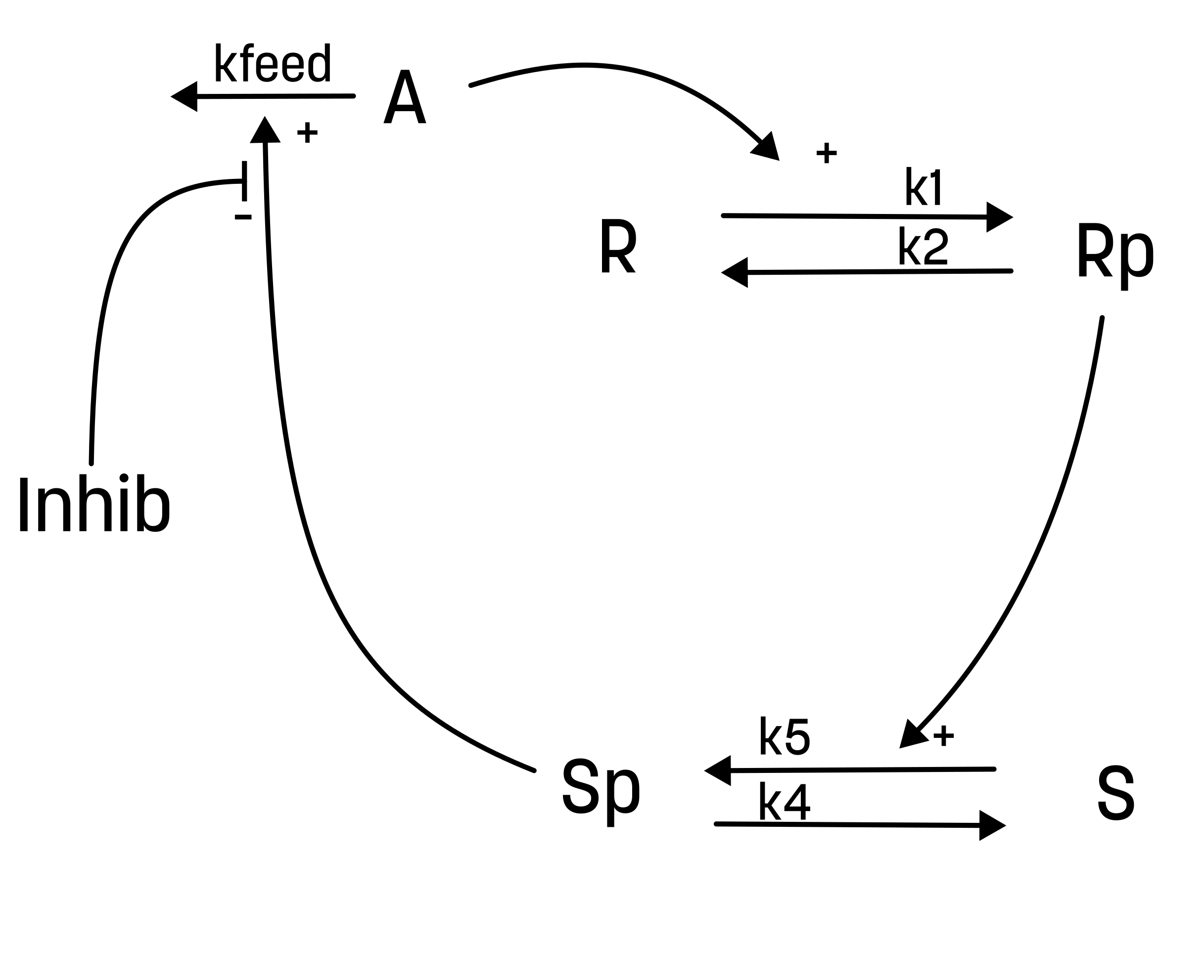
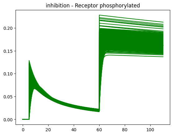
Here, the inhibition is not absolute. Rather, there is an increasing effectiveness of increasing the concentration of the inhibitor. To easier vizualize the efffect, the inhibitor should be introduced when the second dose of the training data occurs t = 60 and have no effect during the first response.

The inhibition could in a simple way be interpretated as: r3 = kfeed*A*Sp*(1/inhibitor)

Start by implementing the new model.

Implement an inhibition to the elimination of A

The interaction of the inhibition could be presented as below. Note that this model structure just adds a new input but otherwise is the same as the second hypthesis.

Start by creating a new text file. We assume that you name this model M2_inhib.

The inhibitatory substance could be called inhibitor and should be introduced with an event.

...

########## EVENTS
input_event = inhibitor>0 
########## OUTPUTS
########## INPUTS
inhibitor = inhibitor_in @ 1.0

Define the inhibition activity

Now, you will need to define two activities. 1) for the behavior of A_in and one for the behavior of inhibitor_in and both of these need to be a part of the simulation object. You can assume that the value of inhibitor is set to 100 at t=60. To avoid division with 0 (and to have no effect if there is no inhibitor added), you can have the default value of inhibitor to be 1.

Plot the model uncertainty using the inhibited model

Write a new plot function that takes the following inputs

• all_params (a list of paramer values)
• sims (a dictionart containing simulation object(s))
• timepoints (the time vector to simulate)
• color='b' (a default value for line color)
• n_params_to_plot=500 (the number of parameters to plot)

Build this function so that it takes the gathered parameter values for the second hypothesis and simulates the inhibited version with these parameters.

What does the prediction of the inhibition effect tell you?

(spoilers) Self-check: How can I know if the inhibition effect has been implemented correctly?

If implemented correctly, the Rp feature should look something like this.

Checkpoint and reflection

Present the figure with the prediction with uncertainty from both of the models, and how well they agree with the data. Explain if you should reject any of the models based on this figure.

Questions to reflect over

• Did you reject any of the models?
• What are the strengths of finding core predictions that are different between models potentially describing the same system?
• What is the downside to choosing points where there is an overlap between the models to test experimentally, even if the predictions are certain ("narrow")?
• What would be the outcome if it was impossible (experimentally) to measure between 2 and 3 minutes?
• Is our simulation uncertainty reasonable? Is it over- or underestimated?
• What could be problems related to overestimating the uncertainty? To underestimating the uncertainty?
• What should you do when your model can correctly predict new data?

And some questions on the whole exercise to reflect over

1. Look back at the lab, can you give a quick recap of what you did?
2. Why did we square the residuals? And why did we normalize with the SEM?
3. Why is it important that we find the "best" parameter sets when testing the hypothesis? Do we always have to find the best?
4. Can we expect to always find the best solution for our type of problems?
5. What are the problems with underestimating the model uncertainty? And with overestimating?
6. If the uncertainty is very big, how could you go about to reduce it?
7. Why do we want to find core predictions when comparing two (or more) models? What are the possible outcomes if we did the experiment?

The end of the exercise

In the exercise, you should have learned the basics of implementing and simulating models, testing the models using a \(\chi^2\)-test, collecting uncertainty and testing the model by predicting independent validation data. You should now know the basics of what you need to do a systems biology project

This marks the end of the exercise. But, we have also included some additional steps below, which might be relevant for some projects. You can do them now, or come back here later when it is relevant.

Additional exercises (optional)

These are optional to do, but might be relevant in your future projects. Even if you do not do them now, remember that you can come back and try this out later.

Making a profile-likelihood plot

About profile-likelihood

In a profile-likelihood analysis, we plot the value of one parameter on the x-axis and the cost of the whole parameter set on the y-axis. Such a curve is typically referred to as a profile-likelihood curve. To get the full range of values for the parameter, it is common practice to fixate the parameter being investigated, by removing it from the list of parameters being optimized, and setting it explicitly in the cost function, and re-optimize the rest of the parameters. This is done several times, and each time the parameter is fixed to a new value, spanning a range to see how the cost is affected from changes in the value of this specific parameter (Figure 4). If the resulting curve is defined and passes a threshold for rejection in both the positive and negative direction (Figure 4A), we say that the parameter is identifiable (that is, we can define a limited interval of possible values), and if instead the cost stays low in the positive and/or the negative direction, we say that the parameter is unidentifiable (Figure 4B-D). This whole procedure is repeated for each model parameter.

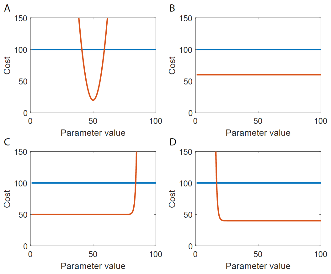Figure 4: Examples of identifiable (A) and unidentifiable parameters (B-D). The blue line is the threshold for rejection, the red line is the value of the cost function for different values of the parameter. In a prediction profile-likelihood analysis, predictions instead of parameter values are investigated over the whole range of possible values. Predictions cannot be fixated, like parameters can. Therefore, the prediction profile-likelihood analysis is often more computationally heavy to perform than the profile-likelihood analysis. Instead of fixation, a term is added to the cost to force the optimization to find a certain value of the prediction, while at the same time minimizing the residuals. Resulting in an objective function something like the following:

\[\begin{equation*} v\left(\theta\right) = \sum_{\forall t}\frac{{(y_t-\ {\hat{y}}_t\left(\theta\right))}^2}{{SEM}_t^2} + \lambda (p - \hat{p}) \end{equation*}\]

Again, the whole range of values of the predictions are iterated through. A prediction profile-likelihood analysis can be used in the search for core predictions.

Do a profile-likelihood analysis of the parameters

Here, we will not fixate one parameter at time and reoptimize, instead we will use the already collected data. This is worse than fixing the parameters, but we will do it for the sake of time. Furthermore, as opposed to the uncertainty plots before, we do not have to select some parameter sets, we can instead use all of our collected sets. The easiest way to do a profile-likelihood plot, is to simply plot the cost against the values of one parameter. Then repeat for all parameters. To make it slightly more pretty, one can filter the parameters to only give the lowest cost for each parameter value. This can be done by first sorting the parameters according to the overall cost, using the function numpy.argsort, and then using the function numpy.unique. A good idea is likely to round your parameter values to something with fewer decimals. This can be done with numpy.round. Note that numpy.round takes an optional argument: decimals which specify the number of decimal to store, can be a negative number.