TBMT42 Lab 1A: Model formulation¶

The purpose of this lab is to learn how to formulate different types of models (ODEs and DAEs) based on previous information about the biological system, and how to analyze the different behaviours in the resulting model.

Throughout the lab you will encounter different "admonitions", which as a type of text box. A short legend of the different kinds of admonitions used can be found in the box below:

Different admonitions used (click me)

Background and Introduction

Useful information

Guiding for implementation

Here you are tasked to do something

Reflective questions

Before you start with this lab, you are expected to have:

Python installation running on your computer (or a computer in the computer hall)
Python packages, including the SUND package. All packages required for this lab is found in requirements.txt.
A C-compiler installed
Downloaded and extracted the scripts for Lab 1.1: Lab1.1 files

If you haven't done this, go to Get started and follow the instructions before you start with this lab.

Note: This module is python-based. You are free to use any software, however, if you don't use Python you will need to redo the pre-made scripts yourself.

Create a mathematical model of fat metabolism¶

In systems biology, one common problem is to go from a scientific question about the mechanisms of a biological system, such as the fat metabolism, to formulating a mathematical model. Here, you are set to formulate, simulate, and analyze a mathematical model of the fat metabolism based on a hypothesis of how the metabolism works.

All files needed in this example are located in the folder fatMetabolism inside the Lab1A files.

Formulate the model¶

First, we formulate the mathematical model.

Task 1: Formulate the mathematical model of fat metabolism

1.1: Read the model description
1.2: Formulate the model equations in a SUND model file

1.1: Click to expand the hypothesis description

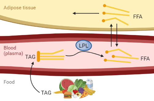
Figure 1: Hypothesis of fat uptake from a meal. Created with BioRender.com

Figure 1 describes the hypothesis of fat uptake during a meal. We are interested in the dynamics of triglycerides (TAG) and free fatty acids (FFA). TAG consists of three FFA and one glycerol, and it is in this form that fat usually is stored in food and in the body. FFA is released when the body needs to utilize the energy from the fat - either to store it in another place or to use it as energy source.

All concentrations of meal-derived TAG and FFA in the body are 0 before the meal. The meal starts at time 1 and consists of 6000 \(\mu\)mol TAG.

The TAG from the meal is taken up in the blood with a rate of 0.015 min\(^{-1}\).

The TAG in the blood is then hydrolysed by the enzyme lipoprotein lipase (LPL), that cleaves the TAG into three FFA. The action of LPL is saturated by the concentration of TAG in the blood (\(TAGp\)) and can be described by Michaelis Menten kinetics, where the limiting rate \(Vmax = 17 \mu mol/L/min\) and the Michaelis Menten constant \(km = 100 \mu mol/L\): \(vLPL = \frac{Vmax*TAGp}{km+TAGp} \mu mol/L/min\).

The FFA in plasma can be transported into the adipose tissue through diffusion. The diffusion rate kd is assumed to be 0.08 min\(^{-1}\). The concentration of FFA that is transported from plasma to adipose tissue and the other way around is dependent on the FFA concentrations in tissue and plasma, as well as the volumes in the tissue and plasma respectively. The plasma volume is approximated to 3 L and the volume of adipose tissue is 1.2 L.

Finally, the FFA in the adipose tissue can be stored and utilized inside the adipose tissue, and this happens with a reaction rate around 1 min\(^{-1}\).

The concentration of both TAG and FFA in plasma after a meal are expected to increase quickly after the meal, to then decrease as the TAG is cleaved into FFA and the FFA is taken up and utilized in the tissue. The meal response is expected to last up to 6 hours (360 minutes) until the fat from the food is fully taken up in the tissues.

1.2: Implement model equations based on the interaction graph

When you have read the hypothesis and looked at the interaction graph, the next step is to translate the interaction graph into equations, in this case ordinary differential equations (ODE). Create a text file and write down the equations in the following SUND format. Save the file as fat_model.txt.

Make sure that the name in the model file is the same as the name of the model file (fat_model).

For more information on the SUND toolbox, see the SUND documentation

Equation format

The text file with the model equations (model file) should have the following format (see ExampleModel.txt): Note that the text file must contain all headers (beginning with “########## “)

########## NAME
ExampleModel
########## METADATA
timeunit = m
########## MACROS
########## STATES
d/dt(A)= r1 - r2                                                   

A(0) = 1
########## PARAMETERS
k1 = 1
k2 = 5
########## VARIABLES
// This is a comment
r1 = k1
r2 = A*k2

variable1 = A*10
########## FUNCTIONS
########## EVENTS
event1 = A_in > 0, A, A_in // event to set A to A_in
########## OUTPUTS
########## INPUTS
A_in = A_in @ 0 // @ 0 means that A_in has the value 0 if A_in is not given as input
########## FEATURES
A measured = variable1 # unit of variable1

How to model food uptake

You can implement the food uptake as follows:

d/dt(TAGfood) = -vfatUptake
TAGfood(0) = 0
vfatUptake = TAGfood*kf

Where TAGfood is the amount of triglycerides that the food contains in \(\mu\)mol, \(vfatUptake\) is the reaction of TAG transferred from the food into the blood, and \(kf\) is a parameter describing the rate of food uptake in min\(^{-1}\).

To input a meal with a certain amount of food, an input food_in can be used:

food = food_in @ 0 // @ 0 means that food has the value 0 if `food_in` is not given as input

together with an event that sets the state TAGfood to the amount specified by the input:

event1 = food > 0, TAGfood, food

Note: Since the TAG in plasma is expressed as a concentration (\(\mu mol/L\)) and not just an amount in \(\mu mol\), the uptake of food into plasma is dependent on the volume of the plasma: \(foodUptake/Vplasma\).

How to model diffusion

FigureDiff

Figure: Zoomed in hypothesis of the diffusion reaction. Created with BioRender.com

One can think of diffusion as two reactions happening at the same time: one reaction \(vd1\) transporting FFA from the plasma to the tissue, and one reaction \(vd2\) transporting FFA from the tissue to the plasma. Both reactions have the same diffusion rate \(kd\) min\(^{-1}\), and the net diffusion, ie the sum of vd1 and vd2, is only dependent on the difference between the concentration of FFA in plasma FFApand the concentration of FFA in tissue FFAt.

The net diffusion rate vnetDiffusion (\(\mu\)mol/L/minute) in the direction from plasma to tissue can thus be calculated as vd1-vd2: \(kd*FFAp - kd*FFAt\).

However, since we have the states in the unit of concentration and the tissue has a smaller volume than the plasma, the reaction rate of the diffusion from tissue to plasma in the ODE of FFAt needs to take the ratio between the volumes Vplasma and Vtissue into consideration.

Note: Remember that in the conversion from TAG to FFA, the LPL reaction results in 3 FFA for every TAG.

Model features

The model features should contain everything from the model that you are interested in, such as state values or variables. The model features can have longer, more descriptive names, and can also have units. Some interesting features to start with, to be able to double check that you have implemented the model correctly, are the four states and four reactions in the model:

########## FEATURES
TAG in food = TAGfood # umol
TAG in plasma = TAGp  # umol/L
FFA in tissue = FFAt  # umol/L
FFA in plasma = FFAp  # umol/L

LPL reaction rate = vLPL # umol/L/min
Fat uptake rate = vfatUptake # umol/min
Fat utilization rate = vFatUtalization  # umol/L/min
Net diffusion rate = vnetDiffusion  # umol/L/min

But you will add more features as you go along in the lab.

Was the model you created correctly implemented? A first step to check this is to simulate the model and visually inspect if the simulation behaves as expected.

Task 2: Simulate the created model

To simulate and plot the model, we will use the given script mainFat.py where you will add functions to plot and simulate the model. In this task, we will start by creating a simulation:

2.1: Install and import the model
2.2: Create simulation and activity objects
2.3: Simulate the model

2.1: Install and import the model

Open the script mainFat.py. From this script, we will call all other functions needed to simulate and analyze the model.

To be able to simulate the model, we first need to install it so that it can be used by python. To install your model, you use the SUND package function installModel("filename"). This will basically define a new model class which contains the mathematical model. This class can then be imported and used to create model objects. Now, install the model.

In the mainFat.py script, add code to install your model:

# Install the model by using the sund function 'installModel'
# To verify that the model has been installed try running 'installedModels' afterwards
sund.installModel('fat_model.txt')
print(sund.installedModels())

Once a model has been installed it can be imported to Python. To do this use the sund function importModel(modelname) (with the model name given in the model file). The function will return a model class which should be stored in variable, say M.

In the mainFat.py script, add code to import your model:

# Import the model by using the sund function 'importModel'
M = sund.importModel('fat_model')

To create a model object from the M1 model class, call the class constructor as follows:

In the mainFat.py script, add code to create a model object:

# Create a model object by calling the class constructor '()'
fat_model = M()

A new model object is now stored in the variable fat_model.

Note that the parameter and state values of the model object defaults to what was written in the model file when it was installed. This means that if you change the values in the text file without reinstalling the model, nothing will happen.

When you have installed and imported the model, it is time to create activity and simulation objects to be able to simulate the model.

2.2: Create simulation and activity objects

To simulate the food intake starting at time 1, we first set the initial condition of the state \(TAGfood\) to the amount of fat that the food contains (6000 \(\mu\)mol, see hypothesis description). This is defined as an input 'food_in' in the model file.

Inputs can either be output from other models, or from an activity object. Here, the model needs an input "food_in", which we will now give as an output from a custom activity object.

Note that an activity can have multiple outputs, which are added to the activity object by using the .AddOutput function:

In the mainFat.py script, add code to create an activity object:

# Create activity which sets the food input to 6000 at time 1
activityFood = sund.Activity(timeunit='m')
activityFood.AddOutput(sund.PIECEWISE_CONSTANT, "food_in", tvalues = [1], fvalues=[0,6000])

The simulation of models is carried out by a simulation object, which can include one or more model objects, and (optionally) one or more activity object. To create a simulation object, call the class constructor Simulation from the SUND package. You will need to provide the model objects that should be included when you do the constructor call.

In the mainFat.py script, add code to create a simulation object:

# Create simulation objects: create a dictionary containing your simulation object (optional, but recommended if you have several simulation objects)
sims = {} # Create an empty dictionary
sims['Original model'] = sund.Simulation(models = fat_model, activities = activityFood, timeunit = 'm') # create a new simulation object and add it to the dictionary

2.3: Simulate the model

Now, it is time to perform a model simulation. The simulation object has a function Simulate which can be used to perform a simulation. The simulation needs the time points to simulate (a list of points), and the unit of the time points ('s' for seconds, 'm' for minutes, 'h' for hours).

In the mainFat.py script, set time to a vector in minutes and load the parameter values. :

The time should start at 0, and end at a time that is long enough time to see the meal response.

# Settings for the simulation
timepoints = np.arange(0, 400, 1) # Time in minutes (starting at  t=0 and ending at t=400, with steps of 1)
params = copy.deepcopy(fat_model.parametervalues) # Load parameter values from the model object, as they were defined when the model was installed

Then, use the Simulate function and your simulation object sims['Original model'] to get the simulation.:

# Do a simulation
print(f"Simulation state values before simulation: {sims['Original model'].statevalues}")
sims['Original model'].Simulate(timevector = timepoints,
            parametervalues = params,
            resetstatesderivatives = True)
print(f"Simulation state values after simulation: {sims['Original model'].statevalues}")

The simulation object will store the simulation result for every feature specified in the model file/files, i.e. everything specified under the ########## FEATURES cell. The result is stored in an attribute called featuredata where each column represent one feature, thus the first feature can be accessed using featuredata[:,0]. You can get the feature names using the attribute featurenames.

# Print the feature values from the simulation above. The feature values are stored in the simulation object:
print(f"Values after the simulation: {sims['Original model'].featuredata[:,0]}")
print(f"featurenames: {sims['Original model'].featurenames}")

Are the model and the simulation implemented correctly?

If the model is correctly installed, the following output should be generated:
```
Model 'fat_model' successfully installed.
```
or, if the model already is installed:
```
Model 'fat_model' is already installed and up to date.
```
If the model equations and inputs are correctly implemented, the state values after a simulation of 400 minutes should be:
```
Simulation state values after simulation: [15.32548928  0.49736232  4.90343899  0.82760139]
```
(The order of the states is: TAGfood, TAGp, FFAp, FFAt)

Tip: if the model is not correctly implemented, and you cannot find what is wrong after going through all the above steps again, it could help to go to the next step and plot the simulation. Then, one can see if the features behaves as expected (and which that don't).

Analyze the model¶

Using the simulation object, we can now plot and analyze the model features.

Analyze the model simulations¶

Task 3: Plot and analyze the model simulations

In this task, you should create the following plots:

3.1: Plot an overview of all features in the model
3.2: Plot the diffusion reactions
- Check 1: is the sum of the amounts constant over time?
- Check 2: do the concentrations remain constant if they start at equal values?
3.3: Plot the LPL reactions
- Change the value of Vmax, and plot the LPL reactions again
- Change the value of Km, and plot the LPL reactions again

Note: For each plot task, there is a prepared python function available for you in the main script in the Lab1A files.

First, we will plot and analyze the general behaviour of the model.

3.1: Plot an overview of all features in the model

Call the function ´plot_features´ from your main script to plot all features in the model. ´plot_features´ takes (params, sims, timepoints, figname='', features_to_plot = [], c = 'b') as inputs but does not return any outputs:

sequenceDiagram
Main ->> plot_features: params, sims, timepoints, figname = '', features_to_plot = [], c = 'b'
plotSimulation ->> Main: [ ]

The last arguments (figname,features_to_plot, and c) are optional. If an optional argument is not provided, the default value is used. If the argument features_to_plot is not provided, all features defined in each simulation object in the sims dictionary are plotted. For now, you do not need to provide the optional arguments, but if you want you could add a figure name to know what you are plotting:

plot_features(params,sims,timepoints,figname='All features')

Look at the plot with all the model features. How does the meal response look? Is it reasonable compared to the hypothesis?

Sanity check: If the model is implemented correctly, the following questions should be answered with a yes

Is the TAG in the food disappearing as it is taken up into the blood?
Does the TAG and FFA in the blood increase directly after the meal?
Is the fat utilized by the body? (is it disappearing from the tissue?)

Note: If you detect any errors in your model formulation and make changes in the model file, you need to re-install and re-import the model. It might be a good habit to always install and import the model before you do any simulations.

To further analyze the diffusion and LPL reactions, we will specifically plot their reaction rates.

3.2: Plot and analyze the diffusion reactions

When analyzing the diffusion reaction, we want to add some extra features to be able to double check that it is implemented correctly. We will add the following features to the model file (you need to provide the equations for each feature yourself):

// Extra features to examine the diffusion reaction:
Net diffusion amount =   # umol/min  // amount of FFA per minute between the tissue and plasma

Diffusion rate to plasma = -vnetDiffusion  # umol/L/min  //the diffusion reaction rate in the ODE of FFAp
Diffusion rate to tissue =   # umol/L/min //the diffusion reaction rate in the ODE of FFAt
Diffusion amount to plasma =  # umol/min  // the corresponding amount/minute (remember that concentration*volume = amount)
Diffusion amount to tissue =  # umol/min // the corresponding amount/minute (remember that concentration*volume = amount)

# FFA in tissue =  # umol // amount of FFA in tissue (remember that concentration*volume = amount)
# FFA in plasma =  # umol // amount of FFA in plasma (remember that concentration*volume = amount)
Sum of #FFA in tissue and plasma =  # umol // sum of the two features above

Call the function plot_features with the extra optional argument features_to_plot containing a list of selected features from your main script to plot the reactions connected to the diffusion:

features_to_plot = ['Net diffusion rate', 'Net diffusion amount',
            'Diffusion rate to tissue','Diffusion rate to plasma',
            'Diffusion amount to tissue','Diffusion amount to plasma']
plot_features(params,sims,timepoints,figname='Diffusion',features_to_plot=features_to_plot)

Look at the diffusion plots.

Which way does the net diffusion go to? Does this make sense?
Is the reaction rate of FFA diffusing into the tissue the same as the reaction rate of FFA diffusion from tissue to plasma? If yes, go back to your model formulation of the diffusion reactions! (why?)

Check 1 of the diffusion reaction: is the simulation of #FFAp+#FFAt constant over time?

One test to check that the diffusion is implemented correctly is to check that the sum of the amounts of FFA in tissue and amounts of FFA in plasma is constant over time, when removing all other inputs and outputs.

In the fat model, we have an output from tissue - fat utilization -, and one input to plasma - the LPL reaction - which we need to set to 0 to be able to perform the check.

We also need to set the initial conditions for the states FFAt and FFAp to non-zero the make sure we see the effect.

# Remove all inputs and outputs except the diffusion
# assumes that the parameter governing the fat utilization is named ku and that the Vmax parameter is called vmax
params[fat_model.parameternames.index('ku')] = 0 #turn off the fat utilization
params[fat_model.parameternames.index('vmax')] = 0 #turn off the LPL reaction
# Set non-zero initial concentrations
fat_model.statevalues[fat_model.statenames.index('FFAp')] = 100
fat_model.statevalues[fat_model.statenames.index('FFAt')] = 200

Now, we can select some interesting features and plot them:

# Plot the simulated diffusion features
features_to_plot = ['Net diffusion rate', 'Net diffusion amount',
                    '# FFA in tissue','# FFA in plasma',
                    'FFA in tissue','FFA in plasma', 
                    'Sum of #FFA in tissue and plasma']
plot_features(params,sims,timepoints,figname='Diffusion - check 1',features_to_plot=features_to_plot)

Run the mainFat script again, and look at your new plot.

Look at the diffusion plots from check 1

Is the sum of the amounts of FFA in plasma and FFA in tissue constant over time? If not, go back to your model formulation of the diffusion reactions! (why?)

Check 2 of the diffusion reaction: if [FFAp] = [FFAt], will they remain constant?

A second test to check that the diffusion is implemented correctly is to check that the concentrations of FFA in tissue and of FFA in plasma are constant over time, when starting at equal concentrations and removing all other inputs and outputs.

(No change in concentration should occur since the diffusion only is driven by the difference in concentration between the two states)

Again, we need to set to reaction rates of fat utilization and LPL to 0.

We also need to set the initial conditions for the states FFAt and FFAp to equal, non-zero, values.

# Remove all inputs and outputs except the diffusion
params[fat_model.parameternames.index('ku')] = 0 #turn off the fat utilization
params[fat_model.parameternames.index('vmax')] = 0 #turn off the LPL reaction
# Set equal, non-zero, initial concentrations
fat_model.statevalues[fat_model.statenames.index('FFAp')] = 200
fat_model.statevalues[fat_model.statenames.index('FFAt')] = 200

Now, we can select some interesting features and plot them:

# Plot the simulated diffusion features
features_to_plot = ['Net diffusion rate', 'Net diffusion amount',
                    '# FFA in tissue','# FFA in plasma',
                    'FFA in tissue','FFA in plasma', 
                    'Sum of #FFA in tissue and plasma']
plot_features(params,sims,timepoints,figname='Diffusion - check 2',features_to_plot=features_to_plot)

Run the mainFat script again, and look at your new plot.

Look at the diffusion plots from check 2

Is the concentrations of FFAp and FFAt constant over time? If not, go back to your model formulation of the diffusion reactions! (why?)

Note: Before continuing, remember to set the reaction rates and state values to their original values again!

# Before continuing, reset the model state values to 0 and the parameter values to their model values
fat_model.statevalues[fat_model.statenames.index('FFAp')] = 0
fat_model.statevalues[fat_model.statenames.index('FFAt')] = 0
params = copy.deepcopy(fat_model.parametervalues) # Load parameter values from the model file

3.3: Plot and analyze the LPL reactions

Call the function plot_LPLkinetics from your mainFat script to plot the reactions connected to the diffusion. plot_LPLkinetics takes (params, sims, timepoints, plotfeatures = ['vLPL', 'TAG in plasma']) as inputs but does not return any outputs:

sequenceDiagram
Main ->> plotLPLkinetics: params, sims, timepoints, plotfeatures = ['vLPL', 'TAG in plasma']
plotLPLkinetics ->> Main: [ ]

The first argument params is a list of the parameter vectors corresponding to the simulation objects in the sims dictionary.

The last argument plotfeatures is optional, and should contain a list of the names of the feature for the reaction of LPL (which per default is called vLPL) and the feature for the state TAG in plasma (which per default is called TAG in plasma). These names need to correspond to the feature names in your model file.

A call to the plot function with one object in the sims dictionary could look like:

plot_LPLkinetics([params],sims,timepoints,figname='')

Look at the plot of the velocity of the LPL reaction vs the concentration of the substrate TAG in plasma.

Can you find the substrate concentration where the velocity is half of Vmax? What parameter does that velocity correspond to?
Does the rate of the LPL reaction ever reach Vmax?
Compare to the plot of the LPL reaction vs time and the plot of the concentration of TAG in plasma vs time - can you find the corresponding time point where the velocity is Vmax/2?
Change the value of the km parameter (eg to 10 or 1000 instead of 100), make a new figure of the LPL kinetics using the pre-defined plot function, and re-run the main script. How does that affect the plot of LPL kinetics?
```
# assumes that the km parameter is named km in the model file
params[fat_model.parameternames.index('km')] = 10 # change the MM kinetics by changing km
plot_LPLkinetics([params],sims,timepoints,figname='km = 10')
```
Change the value of Vmax (eg to 30 or 10 instead of 17) and re-run the main script. How does that affect the plot of LPL kinetics?

Analyze different kinetics for the LPL reaction¶

To see how the model formulation affects the model simulation, we can change the kinetics of the LPL reaction and se how that affects the reaction rate.

Task 4: Change the kinetics of the LPL reaction

Sometimes one needs to try different types of kinetics for the reactions to see which kinetics that is needed to be able to describe the biological system and agree with data. Now, change the kinetics for the LPL reaction to see how the dynamics of the meal response changes.

Change the dynamics to the following kinetics and plot the results:

4.1: Mass action kinetics
4.2: Hill kinetics, with different values for n

Different types of kinetics

There are several types of kinetics that can occur in biological systems. Here, we will cover thee of the most common examples:

Mass action kinetics is the most basic type of kinetics, where the reaction rate \(v\) is directly proportional to the concentration of the reactant \(A\): \(v = k*[A]\)

Michelis Menten kinetics describes a reaction rate \(v\) that is saturated when there is a lot of substrate, and was originally used to describe enzyme kinetics. The Michaelis Menten kinetics can be expressed as: \(v = \frac{Vmax*[A]}{k_{m}+[A]}\) where the reaction rate \(v\) is saturated at the limiting rate \(Vmax\) if there is enough substrate \(A\). The Michaelis Menten constant \(k_{m}\) corresponds to the substrate concentration where the reaction rate is half of \(Vmax\).

Hill kinetics describes a sigmoidal response and was originally used to describe the binding of oxygen to hemoglobin in the blood. Hill kinetics can be used to describe receptor-ligand or enzyme-substrate kinetics in biochemistry or pharmacology. The Hill equation can be expressed as: \(v = \frac{Vmax*[A]^{n}}{k_{a}^{n}+[A]^{n}}\) where \(k_{a}\) is the substrate concentration where \(v = Vmax/2\) and the inflection point of the sigmoid response is found. The Hill coefficient \(n\) governs the sensitivity to the amount of substrate A: if \(n\) > 1 the binding of one substrate facilitates binding of more substrates, but if \(n\) < 1 the binding of one substrate reduces the affinity for other substrates. What happens when \(n\)=1?

4.1: Change the kinetics of LPL to mass action kinetics

Create a copy of your model file fat_model.txt, and name it fat_model_massAction.txt. In your new model file, update the model name and change the reaction vLPL from Michaelis Menten kinetics to mass action kinetics.

In your mainFat.py script, add code to install and import the model, create a model object, and create and add a simulation object to the simulation dictionary. The new simulation object can be called 'Massaction'.

Use the plot_LPLkinetics function to plot the results. Now, include parameters for all your simulation objects.

plot_LPLkinetics([params,massactionparams],sims,timepoints)

Run the main script to generate the resulting plots.

Now, we are only interested in the new plots of the LPL kinetics. If you want, you can comment out the lines that call the plot functions in Task 3 by adding a # before each line.

How does the meal dynamics change?

Look at the plot of the LPL kinetics. What is the difference between Michaelis Menten and mass action kinetics?

4.2: Change the kinetics of LPL to Hill kinetics

Create a copy of your original model file fat_model.txt, and name it fat_model_Hill.txt. In your new model file, update the model name and change the reaction vLPL from Michaelis Menten kinetics to Hill kinetics by adding the Hill coefficient \(n\): \(vLPL = \frac{Vmax*TAGp^{n}}{km^{n}+TAGp^{n}}\)

First, set n = 3. Then, try at least two other values for \(n\): one where \(n<1\) and one where \(n=1\).

In your mainFat.py script, add code to install and import the model, create a model object, and create and add a simulation object to the simulation dictionary. The new simulation object can be called 'Hill'.

Remember to also add your new parameter vector (maybe called hillparams).

Run the main script to generate the resulting plots.

How does the meal dynamics change?

Look at the plot of the LPL kinetics.

What is the difference between Hill, Michaelis Menten, and mass action kinetics?
How does the value of the Hill coefficient \(n\) affect the kinetics?

Create a mathematical model of the cardiovascular system¶

Not all systems can be described using ordinary differential equations - there are several other types of equations that might be needed for different systems. In this example, to model the cardiovascular system, we need to add algebraic equations with time-varying variables without their derivatives. Thus, in this example we will use differential algebraic equations (DAE) instead of ODEs.

Differential algebraic equations (DAE)

DAEs are equations where ordinary differential equations are not enough to describe the system. Instead, additional algebraic equations are needed, which contain other time-dependent variables without their derivative:

\(F(x'(t),x(t),t) = 0\)

\(x'(0) = x'_{0}\)

\(x(0) = x_{0}\)

where \(x\) not only contains the state of the model but also other variables.

DAEs appear in many situations, such as electrical circuits, chemical processes, or mechanical systems like the motion of a pendulum.

The initial conditions of both \(x(t)\) and \(x'(t)\) can be set in DAEs. However, the initial conditions always need to be consistent with the equations you are solving, which can be especially tricky in DAEs. There are helper functions to find consistent initial conditions as close as your wanted ones as possible, and some solvers do this automatically.

Note: Some DAEs (ie with low differential index*) can easily be re-written as ODEs and solved with ODE methods - but not all.

*Differential index: The minimum number of times the DAE has to be differentiated to get an ODE. A semi-explicit DAE with index 1 could be defined as \(x'(t) = f(x(t),y(t),t), 0 = g(x(t),y(t),t)\). Be aware of that if a DAE is differentiated, the constrains might disappear.

All files needed in this example are located in the folder cardiovascularSystem inside the Lab1A files.

Cardiovascular models

Electrical circuits are often used as an analogy when creating models of the cardiovascular system, where the cardiovascular fluid dynamics are represented by electrical components: the blood flow is represented by a current I, pressure differences by a voltage V, vessel resistance by a electrical resistance, compliance of elastic vessels by conductance, and the inertia of the blood by inductance. Thus, by drawing an interaction graph of a simple circuit representing a part of the cardiovascular system, one can use electrical and physical laws such as Kirchhoff's current and voltage laws and Ohm's law to derive mathematical equations of the cardiovascular system.

Cardiovascular fluid dynamics	Electrical circuit

Vessel resistance (R)	Electrical resistance (R)
Blood flow (Q)	Current (I)
Pressure difference (P)	Voltage difference (U)
Compliance (distensibility) of elastic vessels (C)	Capacitance (C)
Blood inertia (L)	Inductance (L)

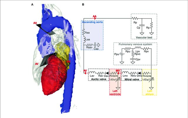
Figure 2. An example of a cardiovascular model from Casas et al 2018, where each part of the heart to the left corresponds to a part in the electrical circuit to the right.

Formulate the model¶

Based on a description of the cardiovascular model, we will formulate the model equations.

Task 5: Implement the model equations of a simple model of the cardiovascular system

Create the model file cardiovascular_model.txt, and write down the model equations, parameters, variables, inputs, and features using the SUND format.

Click to expand the model description

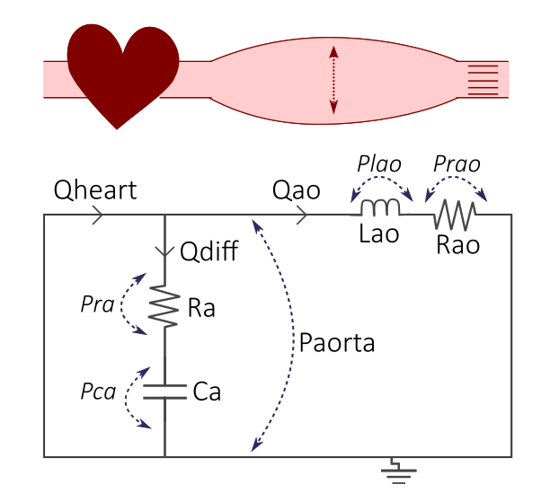
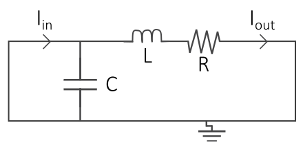
Figure 2. The cardiovascular model, where the cardiovascular system with the heart and elastic aorta (top) is represented by an electrical circuit (bottom).

This simple model represents the blood flow and blood pressure in the aorta, where in general:

Q: Blood flow (mL/s)

R: Resistance (mmHg·s/mL), representing the resistance in blood vessels

L: Inertance (mmHg*s\(^{2}\)/mL), representing the inertia of blood flow

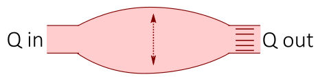
C: Compliance (mL/mmHg), representing the windkessel effect of the aorta which expands and stores blood during systole, and relaxes during diastole

P: Pressure (mmHg)

The input to the model is the length of the cardiac cycle, T (s). T which governs the pattern of the flow input (mL/s) corresponding to the blood flow coming from the heart into the aorta.

Retrieve the equations from the circuit

To retrieve the equations from the circuit, we use electrical and physical laws:

Definition of Ohm's law, inductance, and compliance for each component:
- Ohm's law: \(\varDelta U = R*I <-> \varDelta P = R*Q\)
  - \(Prao = Rao*Qao\)
  - \(Pra = Ra*Qdiff\)
- Inductance: The pressure over the inductance is given as: \(\frac{dP}{dt} = L * \frac{dQ}{dt}\).
  - \(Plao = Lao* \frac{dQao}{dt}\) (Eq L1)
- Compliance: compliance of a vessel defines the stiffness of the vessel - i.e. how much volume change is generated by a change in pressure: \(C = \frac {\varDelta V}{\varDelta P}\). The rate of change in volume over a vessel segment is the blood flow Q ml/s, which gives us: \(Q = C*\frac{dP}{dt}\)
  - \(Qdiff = Ca*\frac{dPca}{dt}\) (Eq C1)
Kirchhoff's voltage law:

All voltages (or blood pressure differences) in a loop should sum up to 0. In this case, we only have one such loop:
- \(Pca + Pra - Plao - Prao = 0\) (KVL1)
Kirchhoff's current law:

All currents (and blood flow) in a node should sum up to 0. In this case, we only have one such node:
- \(Qheart - Qdiff - Qao = 0\) (KCL1)

Finally, we put all the equations together:

Write the ODEs on an ODE format with the derivate to the left:

\(\frac{dPca}{dt} = \frac{Qdiff}{Ca}\) (from Eq C1)

\(\frac{dQao}{dt} = \frac{Plao}{Lao}\) (from Eq L1)

Keep any left over DAEs in the DAE format:

\(Qheart - Qdiff - Qao = 0\) (KCL1, which gives us the value of Qdiff)

\(Pca + Pra - Plao - Prao = 0\) (KVL1, which gives us the value of Plao)

... and the definitons from Ohms law:

\(Prao = Rao*Qao\)

\(Pra = Ra*Qdiff\)

where \(Qheart\) is the input flow.

\(Paorta\) is the aortic pressure, which is a sum of all pressures over the aorta: \(Paorta = Pra + Pca\).

Aortic pressure (with the unit mmHg) is the feature we will look at later.

Look at the equations

Which are the time-varying variables in the model that we will solve for?
Is it possible to re-write the DAEs to ODEs, with one equation defining each derivative, in a simple way?

Read the model hypothesis above, and create the model file cardiovascular_model.txt

Create a model file called cardiovascular_model.txt and write down the model equations from the model description.

Equation format

We use the SUND toolbox to formulate the model. The ODEs are defined in the same way as for the fat model. DAE equations for each algebraeic state AlgebraeicState should be defined on the following format: (see ExampleModelDAE.txt):

########## NAME
ExampleModelDAE
########## METADATA
timeunit = s
########## MACROS
########## STATES
d/dt(A)= r1 - r2
0 = A - AlgebraeicState                                                

A(0) = 1
AlgebraeicState(0) = 5

Initial conditions

The inital conditions need to be coherent, so that all algebraeic equations are fullfilled. Otherwise, the model simulation might crach.

Come up with a coherent initial condition guess for the model. Qheart = 0 at t=0.

Tip: if everything is 0, all equations are fullfilled.

Parameters in the model

The following values for the parameters in the model represent normal values in the cardiovascular system:

Ca =  1.1
Ra = 0.1
Rao = 1.2
Lao = 0.0005

Input Qheart to the model

The input to the model is the blood flow from heart Qheart, which we model as a modified sinus curve:

Qheart = ceil(max(0,k_syst-fmod(time,T)/T))  * 300.*sin((CONSTANT_PI*(fmod(time,T)/T))/k_syst)

In diastole, the heart relaxes and the aortic valve is closed, which means that the blood flow from the heart is 0. This is modelled by the first part of the expression, which is 0 when the valve is closed and 1 when the valve is open. In systole, the aortic valve is open and blood is pumped out, which we model as a sinus curve with the amplitude 300 mL/s.

The parameter k_syst determines the ratio of the length of systole to the length of the full cardiac cycle (T). Here, we set this ratio to k_syst = 0.4.

The cardiac cycle is simulated to start at the start of systole at t=0.

Input T to the model

The length of the cardiac cycle can be defined as an input to the model:

########## INPUTS
T = T_in @ 1 // @ 1 means that T has the value 1 if T_in is not given as input

What is the difference between an ODE and a DAE?

What makes this model a DAE instead of ODE?

Analyze the model¶

When you have written down all the equations in the model file, it is time to simulate the model and plot the results.

Task 6: Simulate, plot, and analyze the cardiovascular model

The given main script already includes the installation and setup of the model, as well as a plot script. Run mainCardiovascular.py to simulate two heartbeats with the model and to plot the resulting simulated blood pressure.

Is the model formulation correct?

If you have correctly formulated the model file, the output from the main script should give you the following values:

Simulation state values after one simulation: [ 5.28647732e+01  4.06761534e+01 -4.06761534e+01 -1.42262586e-02]

(For the states in order: Pca, Qao, Qdiff, Plao)

Look at the resulting plot of aortic pressure

Blood pressure is usually measured as the systolic (the highest value, during systole) and diastolic (the lowest value, during diastole) pressure. What is the systolic and diastolic blood pressure simulated by the model? If the equations are correctly implemented, the systolic pressure should be around 119 mmHg and the diastolic pressure should be around 70 mmHg.

When aging, the blood vessels get stiffer. The stiffening results in a lower compliance of the blood vessels. Do a model prediction of this process by reducing the value of the model parameter Ca and running the mainCardiovascular again.

Look at the resulting plot

In what way did the systolic and diastolic pressure change with the stiffening of the vessels?

Questions for lab 1A¶

In your lab report, you should answer the following questions:

Show your plots of the two sanity checks for the diffusion reaction. Explain how you can tell that the diffusion equations are correctly implemented in your model.
Show one of your plots of Michaelis-Menten kinetics. Describe how the parameters km and Vmax govern the appearance of the plot.
What is the difference between an ODE and a DAE? Use the equations from the two example models from the lab and describe why they are ODEs or DAEs respectively.